大家好，又见面了，我是你们的朋友全栈君。如果您正在找激活码,请点击查看最新教程,关注关注公众号 “全栈程序员社区” 获取激活教程,可能之前旧版本教程已经失效.最新Idea2022.1教程亲测有效,一键激活。

Jetbrains全系列IDE稳定放心使用

前言

记录自己阅读复现SiamFC的全过程，包括论文翻译，代码理解等

一、论文翻译

论文原文：
链接：https://pan.baidu.com/s/1wvXra0Ji6L9IMVZikaUs9Q
提取码：s7t3

本文是Siam系列跟踪论文的开篇之作，兼容了速度与精度，引起跟踪社区极大的关注。论文中对一些细节描述分非常充分，适合精读本文。

二、论文代码

代码参考;
https://github.com/HonglinChu/SiamTrackers/tree/master/2-SiamFC
GOT10k数据集：
链接：https://pan.baidu.com/s/1CtwRPoo9eByqLZUhMTM92g
提取码：5akn

1.网络结构

1.1backbone网络

Alexnet网络

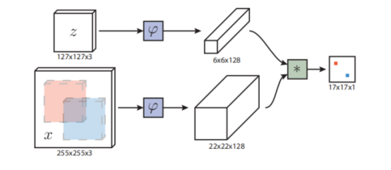
Network architecture. 我们用来进行embedding的函数φ 使用Krizhevsky的卷积阶段。参数和激活函数的维度在Tabel1中给出。在最开始的两个卷积层之后，使用最大值池化。除了conv5和最后一层之外，每个卷积层都使用ReLU。在训练的过程中，batch normalization在每个线性层中插入。最终一层的表示的stride是8。这一设计的重要方面是，在网络中没有引入padding。尽管这在图像分类中很常见，但是它损坏了全卷积的性质。

backbone.py
代码如下：

import torch.nn as nn
__all__ = ['AlexNetV1']
class _BatchNorm2d(nn.BatchNorm2d):
def __init__(self, num_features, *args, **kwargs):
super(_BatchNorm2d, self).__init__(
num_features, *args, eps=1e-6, momentum=0.05, **kwargs)
class _AlexNet(nn.Module):
def forward(self, x):
x = self.conv1(x)
x = self.conv2(x)
x = self.conv3(x)
x = self.conv4(x)
x = self.conv5(x)
return x#返回特征
class AlexNetV1(_AlexNet):
output_stride = 8
def __init__(self):
super(AlexNetV1, self).__init__()
self.conv1 = nn.Sequential(
nn.Conv2d(3, 96, 11, 2),#input 3*127*127 output 96*59*59 
_BatchNorm2d(96),
nn.ReLU(inplace=True),
nn.MaxPool2d(3, 2))#96*29*29
self.conv2 = nn.Sequential(
nn.Conv2d(96, 256, 5, 1, groups=2),#2*128*25*25
_BatchNorm2d(256),
nn.ReLU(inplace=True),
nn.MaxPool2d(3, 2))#2*128*12*12
self.conv3 = nn.Sequential(
nn.Conv2d(256, 384, 3, 1),#384*10*10
_BatchNorm2d(384),
nn.ReLU(inplace=True))
self.conv4 = nn.Sequential(
nn.Conv2d(384, 384, 3, 1, groups=2),#2*192*8*8
_BatchNorm2d(384),
nn.ReLU(inplace=True))
self.conv5 = nn.Sequential(
nn.Conv2d(384, 256, 3, 1, groups=2))#2*128*6*6 

1.2互相关运算

head.py

import torch.nn.functional as F
__all__ = ['SiamFC']
class SiamFC(nn.Module):
def __init__(self, out_scale=0.001):#out_scale，根据作者说是因为， z和x互相关之后的值太大，经过sigmoid函数之后会使值处于梯度饱和的那块，梯度太小，乘以out_scale就是为了避免这个。
super(SiamFC, self).__init__()
self.out_scale = out_scale
def forward(self, z, x):
return self._fast_xcorr(z, x) * self.out_scale
def _fast_xcorr(self, z, x):
# fast cross correlation
#print(z.size())
#print(x.size())
nz = z.size(0)#8*256*6*6
nx, c, h, w = x.size()#8*256*20*20
x = x.view(-1, nz * c, h, w)#1*2048*20*20
#print(x.size())
out = F.conv2d(x, z, groups=nz)
out = out.view(nx, -1, out.size(-2), out.size(-1))#8*1*15*15
#print(out.size())
return out#返回响应图

2.数据集准备

从同一视频中提取训练对：样本图像和同一视频中相应的搜索图像。当子窗口超出图像范围时，丢失的部分将填充平均rgb值。

Dataset curation. 在训练的过程中，我们调整模板图像到127 × 127 ，搜索图像调整到255 × 255 。缩放图像，使边界框加上下文的空白具有固定的区域。更准确地讲，如果边界框的尺寸是（w , h ），上下文的空白是p ，缩放因子是s 被选择用来使尺度调整后的矩形的面积是一个常数s ( w + 2 p ) × s ( h + 2 p ) = A 。使用使用模板图像的面积A= 12 7× 127 。设置上下文的数量为平均维度p = ( w + h ) / 4的一半。每帧的模板和搜索图像被离线提取，为了避免在训练的过程中的resize。在这项工作的初步版本中，我们采用了一些启发式方法来限制从中提取训练数据的帧数。

dataset.py

import numpy as np
import cv2
from torch.utils.data import Dataset
__all__ = ['Pair']
class Pair(Dataset):
def __init__(self, seqs, transforms=None,
pairs_per_seq=1):
super(Pair, self).__init__()
self.seqs = seqs
self.transforms = transforms
self.pairs_per_seq = pairs_per_seq
self.indices = np.random.permutation(len(seqs))
self.return_meta = getattr(seqs, 'return_meta', False)
def __getitem__(self, index):
index = self.indices[index % len(self.indices)]
# get filename lists and annotations
if self.return_meta:
img_files, anno, meta = self.seqs[index]
vis_ratios = meta.get('cover', None)
else:
img_files, anno = self.seqs[index][:2]
vis_ratios = None
# filter out noisy frames
val_indices = self._filter(
cv2.imread(img_files[0], cv2.IMREAD_COLOR),
anno, vis_ratios)
if len(val_indices) < 2:
index = np.random.choice(len(self))
return self.__getitem__(index)
# sample a frame pair
rand_z, rand_x = self._sample_pair(val_indices)
z = cv2.imread(img_files[rand_z], cv2.IMREAD_COLOR)
x = cv2.imread(img_files[rand_x], cv2.IMREAD_COLOR)
z = cv2.cvtColor(z, cv2.COLOR_BGR2RGB)
x = cv2.cvtColor(x, cv2.COLOR_BGR2RGB)
box_z = anno[rand_z]
box_x = anno[rand_x]
item = (z, x, box_z, box_x)#通过index索引返回item = (z, x, box_z, box_x)，然后经过transforms返回一对pair(z, x)
if self.transforms is not None:
item = self.transforms(*item)
return item
def __len__(self):
return len(self.indices) * self.pairs_per_seq#定义的长度就是被索引到的视频序列帧数×每个序列提供的对数
def _sample_pair(self, indices):##如果有效索引大于2个的话，就从中随机挑选两个索引，这里取的间隔不超过T=100
n = len(indices)
assert n > 0
if n == 1:
return indices[0], indices[0]
elif n == 2:
return indices[0], indices[1]
else:
for i in range(100):
rand_z, rand_x = np.sort(
np.random.choice(indices, 2, replace=False))
if rand_x - rand_z < 100:
break
else:
rand_z = np.random.choice(indices)
rand_x = rand_z
return rand_z, rand_x
def _filter(self, img0, anno, vis_ratios=None):#通过该函数筛选符合条件的有效索引val_indices，这里不详细分析，因为我也不知道为什么会有这样的filter condition。
size = np.array(img0.shape[1::-1])[np.newaxis, :]
areas = anno[:, 2] * anno[:, 3]
# acceptance conditions
c1 = areas >= 20
c2 = np.all(anno[:, 2:] >= 20, axis=1)
c3 = np.all(anno[:, 2:] <= 500, axis=1)
c4 = np.all((anno[:, 2:] / size) >= 0.01, axis=1)
c5 = np.all((anno[:, 2:] / size) <= 0.5, axis=1)
c6 = (anno[:, 2] / np.maximum(1, anno[:, 3])) >= 0.25
c7 = (anno[:, 2] / np.maximum(1, anno[:, 3])) <= 4
if vis_ratios is not None:
c8 = (vis_ratios > max(1, vis_ratios.max() * 0.3))
else:
c8 = np.ones_like(c1)
mask = np.logical_and.reduce(
(c1, c2, c3, c4, c5, c6, c7, c8))
val_indices = np.where(mask)[0]
return val_indices

transforms.py
RandomStretch：主要是随机的resize图片的大小，其中要注意cv2.resize()的一点用法
CenterCrop：从img中间抠一块(size, size)大小的patch，如果不够大，以图片均值进行pad之后再crop
RandomCrop：用法类似CenterCrop，只不过从随机的位置抠，没有pad的考虑
Compose：就是把一系列的transforms串起来
ToTensor： 就是字面意思，把np.ndarray转化成torch tensor类型

import cv2
import numpy as np
import numbers
import torch
from . import ops
__all__ = ['SiamFCTransforms']
class Compose(object):
def __init__(self, transforms):
self.transforms = transforms
def __call__(self, img):
for t in self.transforms:
img = t(img)
return img
''' __init__()等同于类的构造器，创建一个类的实例 __del__()等同于类的析构函数 __call__()类的实例可以被当做函数调用 '''
class RandomStretch(object):
def __init__(self, max_stretch=0.05):
self.max_stretch = max_stretch
def __call__(self, img):
interp = np.random.choice([
cv2.INTER_LINEAR,
cv2.INTER_CUBIC,
cv2.INTER_AREA,
cv2.INTER_NEAREST,
cv2.INTER_LANCZOS4])
scale = 1.0 + np.random.uniform(
-self.max_stretch, self.max_stretch)
out_size = (
round(img.shape[1] * scale),
round(img.shape[0] * scale))
return cv2.resize(img, out_size, interpolation=interp)
class CenterCrop(object):
def __init__(self, size):
if isinstance(size, numbers.Number):
self.size = (int(size), int(size))
else:
self.size = size
def __call__(self, img):
h, w = img.shape[:2]
tw, th = self.size
i = round((h - th) / 2.)
j = round((w - tw) / 2.)
npad = max(0, -i, -j)
if npad > 0:
avg_color = np.mean(img, axis=(0, 1))
img = cv2.copyMakeBorder(
img, npad, npad, npad, npad,
cv2.BORDER_CONSTANT, value=avg_color)
i += npad
j += npad
return img[i:i + th, j:j + tw]
class RandomCrop(object):
def __init__(self, size):
if isinstance(size, numbers.Number):
self.size = (int(size), int(size))
else:
self.size = size
def __call__(self, img):
h, w = img.shape[:2]
tw, th = self.size
i = np.random.randint(0, h - th + 1)
j = np.random.randint(0, w - tw + 1)
return img[i:i + th, j:j + tw]
class ToTensor(object):
def __call__(self, img):
return torch.from_numpy(img).float().permute((2, 0, 1))
class SiamFCTransforms(object):
def __init__(self, exemplar_sz=127, instance_sz=255, context=0.5):
self.exemplar_sz = exemplar_sz
self.instance_sz = instance_sz
self.context = context
self.transforms_z = Compose([
RandomStretch(),
CenterCrop(instance_sz - 8),#255-8=247
RandomCrop(instance_sz - 2 * 8),#255-16=239
CenterCrop(exemplar_sz),#127
ToTensor()])
self.transforms_x = Compose([
RandomStretch(),
CenterCrop(instance_sz - 8),#247
RandomCrop(instance_sz - 2 * 8),#239 instance_sz-2 * 8“是在训练阶段使用的255x255图像上的随机裁剪，从而减少了训练数据的过拟合。
ToTensor()])
def __call__(self, z, x, box_z, box_x):
z = self._crop(z, box_z, self.instance_sz)
x = self._crop(x, box_x, self.instance_sz)
z = self.transforms_z(z)
x = self.transforms_x(x)
return z, x
def _crop(self, img, box, out_size):
# convert box to 0-indexed and center based [y, x, h, w]
box = np.array([
box[1] - 1 + (box[3] - 1) / 2,
box[0] - 1 + (box[2] - 1) / 2,
box[3], box[2]], dtype=np.float32)#GOT-10k里面对于目标的bbox是以ltwh(即left, top, weight, height)形式给出的，上述代码一开始就先把输入的box变成center based，坐标形式变为[y, x, h, w]，结合下面这幅图就非常好理解：y=t+h/2,x=l+w/2
center, target_sz = box[:2], box[2:]
context = self.context * np.sum(target_sz)#content=0.5*(h+w)=2p
size = np.sqrt(np.prod(target_sz + context))#np.sqrt((w+2p)(h+2p))
size *= out_size / self.exemplar_sz#255/127*size
#print(size)
#print(box)
avg_color = np.mean(img, axis=(0, 1), dtype=float)#np.mean(img, axis=(0, 1)) 是求出各个通道的平均值
interp = np.random.choice([
cv2.INTER_LINEAR,
cv2.INTER_CUBIC,
cv2.INTER_AREA,
cv2.INTER_NEAREST,
cv2.INTER_LANCZOS4])
patch = ops.crop_and_resize(
img, center, size, out_size,
border_value=avg_color, interp=interp)
#cv2.imshow("image",img)
#cv2.imshow("patch",patch)
return patch

3.训练阶段

Training. embedding函数的参数通过直接的SGD使用MatConvNet最小化函数来实现。参数的初始化使用一个高斯分布，范围遵循Xavier方法。训练使用50个epochs。每个由50000样本对。每次迭代的梯度使用大小为8的mini-batches来估计，学习率每步衰减，从1 0 − 2 到 1 0 − 5

# 在禁止计算梯度下调用被允许计算梯度的函数
@torch.enable_grad()
def train_over(self, seqs, val_seqs=None,save_dir='pretrained'):
# set to train mode
self.net.train()
# create save_dir folder
if not os.path.exists(save_dir):
os.makedirs(save_dir)
# setup dataset
transforms = SiamFCTransforms(
exemplar_sz=self.cfg.exemplar_sz, #127
instance_sz=self.cfg.instance_sz, #255
context=self.cfg.context)  # 0.5 ？？？
dataset = Pair(seqs=seqs,transforms=transforms)
# setup dataloader
dataloader = DataLoader(
dataset,
batch_size=self.cfg.batch_size,
shuffle=True,
num_workers=self.cfg.num_workers,
pin_memory=self.cuda,
drop_last=True)
# loop over epochs
for epoch in range(self.cfg.epoch_num):
# update lr at each epoch
self.lr_scheduler.step(epoch=epoch)
# loop over dataloader
for it, batch in enumerate(dataloader):
loss = self.train_step(batch, backward=True)
print('Epoch: {} [{}/{}] Loss: {:.5f}'.format(epoch + 1, it + 1, len(dataloader), loss))
sys.stdout.flush()
# save checkpoint
if not os.path.exists(save_dir):
os.makedirs(save_dir)
net_path = os.path.join(save_dir, 'siamfc_alexnet_e%d.pth' % (epoch + 1))
torch.save(self.net.state_dict(), net_path)

v是单个模板-候选框对的真值，y ∈ { + 1 , − 1 } 是真值标签。在训练过程中，我们通过使用包含模板图像和较大的搜索图像对来利用网络的全卷积性质。这会产生一个得分图v : D → R ，能够有效地产生许多例子。我们将得分图的损失定义为单个损失的平均值

它对得分图上的每个位置u ∈ D 需要真实标签y [ u ] ∈ { + 1 , − 1 } }。卷积网络的参数θ 由梯度下降法获得。
上面代码是常规操作，具体在train_step里面实现了训练和反向传播：

    def train_step(self, batch, backward=True):
# set network mode
self.net.train(backward)
# parse batch data
z = batch[0].to(self.device, non_blocking=self.cuda)
x = batch[1].to(self.device, non_blocking=self.cuda)
#print("batch_z shape:", z.shape) # torch.Size([8, 3, 127, 127])
#print("batch_x shape:", x.shape) # torch.Size([8, 3, 239, 239])
with torch.set_grad_enabled(backward):
# inference
responses = self.net(z, x)
# print("responses shape:", responses.shape) # torch.Size([8, 1, 15, 15])
# calculate loss计算损失
labels = self._create_labels(responses.size())#？？?
loss = self.criterion(responses, labels)#criterion使用的BalancedLoss，是调用F.binary_cross_entropy_with_logits，进行一个element-wise的交叉熵计算，所以创建出来的labels的shape其实就是和responses的shape是一样的
if backward:#反向传播
# back propagation
self.optimizer.zero_grad() #梯度清零
loss.backward()
self.optimizer.step()#梯度参数更新
return loss.item()

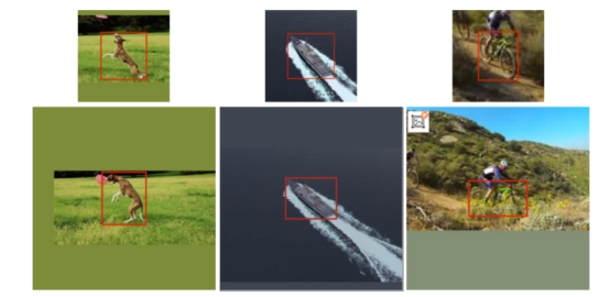
通过在视频标注数据集中提取模板和中心在目标上的搜索图像来获利Pairs,如上图。图像从视频中抽取两帧，它们都包含目标，并且至多相距T 帧。目前的类别在训练的过程中被忽略了。每个图片的尺寸在不破坏图像长宽比的情况下进行标准化。如果得分图的元素在中心的半径R内（考虑网络的步长k ），则认为它们属于正例。
​
得分图中的正样本和负样本的损失被加权，以用来减少类别不均衡的影响。
  因为我们的网络是全卷积的，学习对于中心位置的子窗口偏移是没有风险的。我们相信它能有效考虑目标在中心位置的搜索图像，因为，最困难的子窗口，和那些特别影响追踪器性能的子窗口，是邻近于目标的。

        def _create_labels(self, size):
# skip if same sized labels already created
if hasattr(self, 'labels') and self.labels.size() == size:#用于判断对象是否包含对应的属性
return self.labels
def logistic_labels(x, y, r_pos, r_neg):
dist = np.abs(x) + np.abs(y)  # block distance代表到中心点的距离
#print(dist)
labels = np.where(dist <= r_pos,
np.ones_like(x),#距离小于2的位置是1
np.where(dist < r_neg,
np.ones_like(x) * 0.5,
np.zeros_like(x)))
#print(labels)
return labels
# distances along x- and y-axis
n, c, h, w = size#8,1,15,15
x = np.arange(w) - (w - 1) / 2# [0,1,2...,14]-(15-1)/2-->y=[-7, -6 ,...0,...,6,7]
y = np.arange(h) - (h - 1) / 2#[0,1,2...,14]-(15-1)/2-->x=[-7, -6 ,...0,...,6,7]
x, y = np.meshgrid(x, y)#现根据输入推出输出的shape，然后x一行一行填入，y一列一列按顺序添入就行
# create logistic labels
r_pos = self.cfg.r_pos / self.cfg.total_stride#r_pos=16 total_stride=8#2
r_neg = self.cfg.r_neg / self.cfg.total_stride#r_neg=0#0
labels = logistic_labels(x, y, r_pos, r_neg)
# repeat to size
labels = labels.reshape((1, 1, h, w))
labels = np.tile(labels, (n, c, 1, 1))
# convert to tensors
self.labels = torch.from_numpy(labels).to(self.device).float()
return self.labels

4.推理跟踪阶段

Tracking. 正如前面提到的一样，在线阶段被刻意的简化了。目标的初始外观的embeddingφ ( z ) 只计算一次，在后续帧中，对子窗口以卷积的方式计算。我们发现在线更新模板（特征表示）不能够取得性能的提升，因此，将它保持固定。我们发现，将得分图三次上采样，从17 × 17 到272 × 272 ，能够使定位的结果更准确，因为原始图是相对粗糙的。为了解决尺度变化，我们在四个尺度 1.02 5 { − 2 , − 1 , 0 , 1 , 2 } 1.025^{\{-2,-1,0,1,2\}} 1.025{
−2,−1,0,1,2}上搜索目标，通过线性插值以0.35的系数更新比例以提供减幅。

    def track(self, img_files, box, visualize=False):
frame_num = len(img_files)
boxes = np.zeros((frame_num, 4))
# print(box)
# print(boxes)
boxes[0] = box
times = np.zeros(frame_num)
for f, img_file in enumerate(img_files):
img = ops.read_image(img_file)
begin = time.time()
if f == 0:
self.init(img, box)
else:
boxes[f, :] = self.update(img)
times[f] = time.time() - begin
if visualize:
ops.show_image(img, boxes[f, :])
return boxes, times

@torch.no_grad()
def init(self, img, box):#传入第一帧的标签和图片，初始化参数，计算之后搜索区域的中心
# set to evaluation mode
self.net.eval()
# convert box to 0-indexed and center based [y, x, h, w]
box = np.array([
box[1] - 1 + (box[3] - 1) / 2,
box[0] - 1 + (box[2] - 1) / 2,
box[3], box[2]], dtype=np.float32)
self.center, self.target_sz = box[:2], box[2:]
# create hanning window#计算了响应图上采样后的大小upscale_sz
self.upscale_sz = self.cfg.response_up * self.cfg.response_sz#16*17=272
self.hann_window = np.outer(
np.hanning(self.upscale_sz),
np.hanning(self.upscale_sz))
self.hann_window /= self.hann_window.sum()
# search scale factors
self.scale_factors = self.cfg.scale_step ** np.linspace(#np.linspace(start, stop, num=50, endpoint=True, retstep=False, dtype=None)
-(self.cfg.scale_num // 2),
self.cfg.scale_num // 2, self.cfg.scale_num)
# exemplar and search sizes
context = self.cfg.context * np.sum(self.target_sz)#0.5*（w+h）
self.z_sz = np.sqrt(np.prod(self.target_sz + context))
self.x_sz = self.z_sz * \
self.cfg.instance_sz / self.cfg.exemplar_sz
# exemplar image
self.avg_color = np.mean(img, axis=(0, 1))
z = ops.crop_and_resize(
img, self.center, self.z_sz,
out_size=self.cfg.exemplar_sz,
border_value=self.avg_color)
# exemplar features
z = torch.from_numpy(z).to(
self.device).permute(2, 0, 1).unsqueeze(0).float()
self.kernel = self.net.backbone(z)

@torch.no_grad()
def update(self, img):
# set to evaluation mode
self.net.eval()
# search images
x = [ops.crop_and_resize(#在这新的帧里抠出search images，根据之前init里生成的3个尺度，然后resize成255×255
img, self.center, self.x_sz * f,
out_size=self.cfg.instance_sz,
border_value=self.avg_color) for f in self.scale_factors]
x = np.stack(x, axis=0)
x = torch.from_numpy(x).to(
self.device).permute(0, 3, 1, 2).float()
# responses
x = self.net.backbone(x)
responses = self.net.head(self.kernel, x)
responses = responses.squeeze(1).cpu().numpy()
# upsample responses and penalize scale changes
responses = np.stack([cv2.resize(
u, (self.upscale_sz, self.upscale_sz),
interpolation=cv2.INTER_CUBIC)
for u in responses])
responses[:self.cfg.scale_num // 2] *= self.cfg.scale_penalty
responses[self.cfg.scale_num // 2 + 1:] *= self.cfg.scale_penalty
# peak scale
scale_id = np.argmax(np.amax(responses, axis=(1, 2)))
# peak location
response = responses[scale_id]
response -= response.min()
response /= response.sum() + 1e-16
response = (1 - self.cfg.window_influence) * response + \
self.cfg.window_influence * self.hann_window
loc = np.unravel_index(response.argmax(), response.shape)
# locate target center
disp_in_response = np.array(loc) - (self.upscale_sz - 1) / 2
disp_in_instance = disp_in_response * \
self.cfg.total_stride / self.cfg.response_up
disp_in_image = disp_in_instance * self.x_sz * \
self.scale_factors[scale_id] / self.cfg.instance_sz
self.center += disp_in_image
# update target size
scale = (1 - self.cfg.scale_lr) * 1.0 + \
self.cfg.scale_lr * self.scale_factors[scale_id]
self.target_sz *= scale
self.z_sz *= scale
self.x_sz *= scale
# return 1-indexed and left-top based bounding box
box = np.array([
self.center[1] + 1 - (self.target_sz[1] - 1) / 2,
self.center[0] + 1 - (self.target_sz[0] - 1) / 2,
self.target_sz[1], self.target_sz[0]])
return box

Tracking algorithm. 因为我们的目标是证明全卷积孪生网络的效率和训练在ImageNet video上的泛化能力，我们使用极其简化的算法执行追踪。不像其他的追踪器，我们不需要更新模型或者维持过去的外观变化，我们不需要使用类似于或者颜色直方图之类的额外的线索，我们也不需要使用边界框回来来进行预测的精调。但是，尽管它很简单，使用离线学习的相似度度量仍然达到了令人惊讶的好结果。 我们不需要使用时间限制，我们仅在大约其先前大小的四倍的区域内搜索对象，并将余弦窗口添加到得分图中以惩罚较大的位移。通过处理搜索图像的多个尺度的版本，可以实现对尺度空间的追踪。尺度的任何变化都会受到处罚，当前尺度的更新会受到阻碍。