大家好,又见面了,我是你们的朋友全栈君。如果您正在找激活码,请点击查看最新教程,关注关注公众号 “全栈程序员社区” 获取激活教程,可能之前旧版本教程已经失效.最新Idea2022.1教程亲测有效,一键激活。
Jetbrains全系列IDE使用 1年只要46元 售后保障 童叟无欺
0.前言
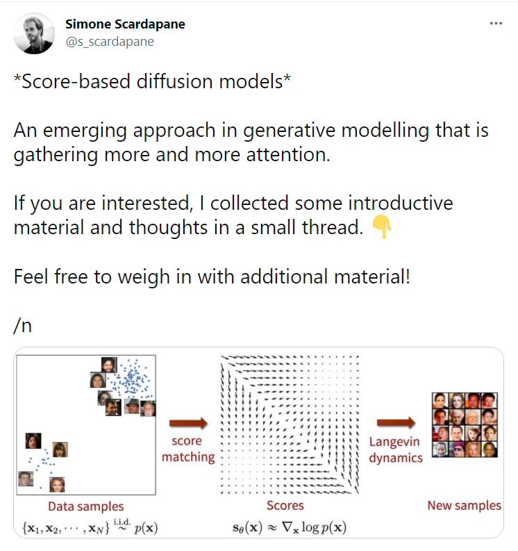
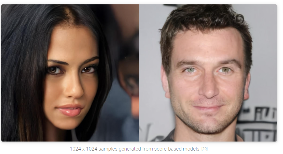
最近(2021.6)发现了生成模型的一种新的trending范式: score-based generative model, 用一句话来介绍这种结构,就是:
通过在噪声扰动后的大规模数据集(noise-perturbed data distributions)上学习一种
score functions (gradients of log probability density functions)(得分函数, 一种对梯度的对数似然估计),用朗之万进行采样得到符合训练集的样本. 这种新的生成模型,叫做score-based generative models (or diffusion probabilistic models)
这种score-based generative model有如下的优点:
- ① 可以得到GAN级别的采样效果,而无需对抗学习(adversarial training)
- ② 灵活的模型结构
- ③ 精确的对数似然估计计算(exact log-likelihood computation)
- ④ 唯一可识别表征学习(uniquely identifiable representation learning)
- ⑤ 流程可逆,我理解是不需要像StyleGAN的模型训练一个feature网络,可能也不需要像FLOW那么大的计算量
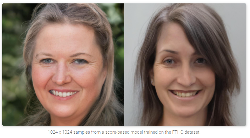
本篇博客的目的,是为了介绍score-based generative model提出的动机,基本概念以及潜在的应用,本文主要翻译自此领域先驱Song Yang博士(斯坦福大学博士)的博客[1]。
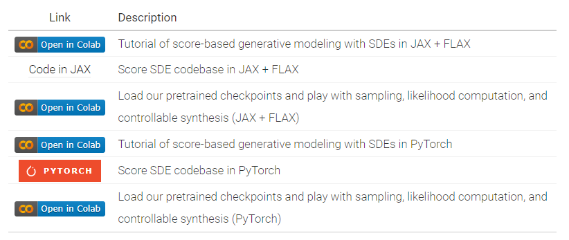
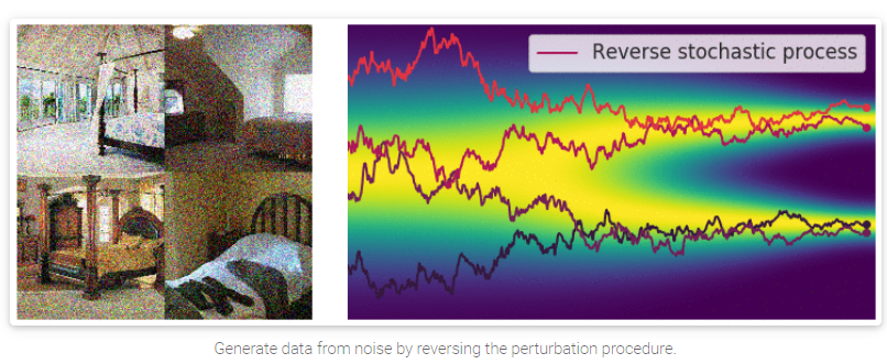
下图来自Twitter用户Simone的分享

1. 介绍
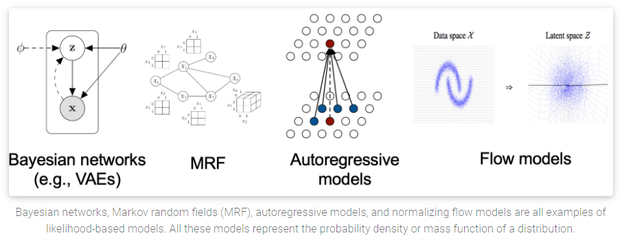
目前,生成模型(generative models)可以根据其表示概率分布的方式主要分为2个大类别:
- likelihood-based models: 通过近似极大似然估计(via (approximate) maximum likelihood)来直接学习分布的PDF(概率密度(D for density)函数)或者PMF(概率质量(M for mass)函数). 典型的基于likelihood的方法有: autoregressive模型
[2], normalizing flow models(如NICE, FLOW等)[3], EBM(基于能量的方法)[4]以及VAE[5].
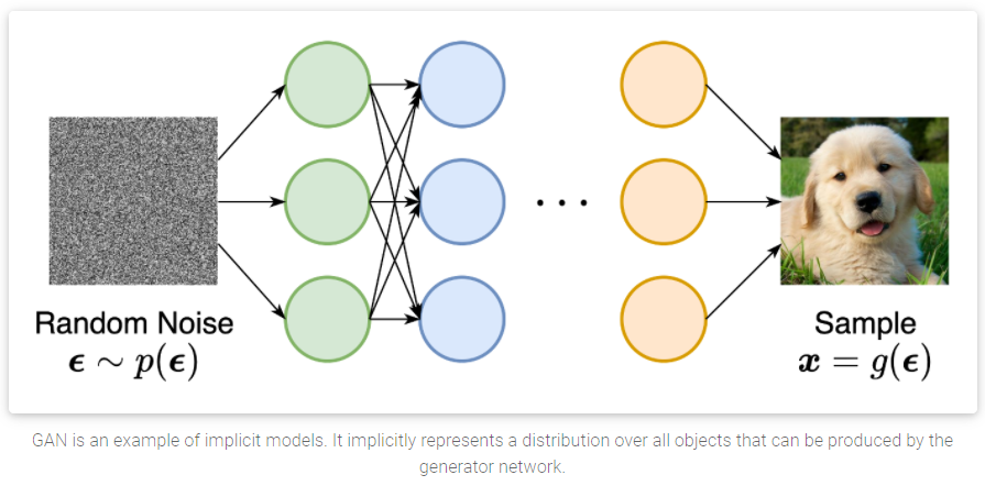
- implicit generative models: GAN中的方法,这种方法的概率分布是通过生成模型的采样过程隐式进行的。GAN中的新样本是通过对随机的高斯向量喂入GAN的生成模型得到的。
这两大类生成模型,都有一些问题: likelihood-based models需要确保易处理的规则化常数(这个后面会提到)以便方便的计算likelihood,而这通常意味着网络结构有较大限制,即无法像NAS那样任意组织和设计网络结构。或者必须依赖于替代的objectives来在训练过程中,近似最大似然(approximate maximum likelihood training). implicit generative models的最大问题是需要对抗训练,而这种训练的方法通常会很不稳定[6]。
本篇博客介绍的就是宋博士提出的score-based generative model, 用这种新的生成模型来解决/规避刚才提到的这些问题。score-based generative model的核心idea是:
对log PDF的梯度进行建模得到一个名为(Stein) score function
[7]的量.
这种score-based generative models不需要处理类似likelihood-based models的规则化常数。而且,score-based generative models在噪声干扰的数据下训练的效果非常好。这类方法可以恢复被噪声干扰的图片本身,并且有着良好的sample quality(采样质量)。
在图像生成[8, 9],音频合成(WaveGrad, DiffWave),形状生成[10],音乐生成都有着良好表现,甚至音频合成领域的效果优于GAN!
当噪声扰动的过程是由 随机可微分方程(stochastic differential equation (SDE)) 给出时, score-based generative models和FLOW这种模型在数学上联系起来了,因此可以进行精确的似然估计计算以及表征学习。
此外,对score的建模以及估计促使其逆向问题得到解决(inverse problem,我想这也是FLOW,NICE等流式模型擅长的地方),这些逆向问题包括:
- image inpainting
[8,9] - image colorization
[9] - 医疗图像重建以及压缩感知等.
2. The score function, score-based models, and score matching
假定我们有一个数据集 x 1 , x 2 , . . . , x N {x_1, x_2, … , x_N} x1,x2,...,xN, 其中的每个 x i , i ∈ 1 , . . . , N x_i, i \in {1, …, N} xi,i∈1,...,N都是从一个潜在的数据分布 p θ ( x ) p_{\theta}(x) pθ(x)中独立取得的(i.i.d). 生成模型的目的是能够完美的建模这个数据分布 p θ ( x ) p_{\theta}(x) pθ(x),以便任意的采样生成符合这个分布的新数据。
为了构造这个生成模型,我们首先需要找到一种可以表示这种概率分布的方式。一种方式就如上面提到的,是likelihood-based models, 即直接对PDF, PMF进行建模。
probability density function (p.d.f.) or probability mass function (p.m.f.)
我们设定, f θ ( x ) ∈ R f_{\theta}(\bf{x}) \in \mathbb{R} fθ(x)∈R是一个以 θ \theta θ为参数的函数。那么,**(p.d.f.)**就可以通过下面的公式定义:
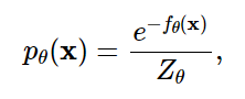
这里, Z θ > 0 Z_{\theta} > 0 Zθ>0是一个依赖于 θ \theta θ的normalizing constant(规则化常数),其目的是让 ∫ p θ ( x ) d x = 1 \int p_{\theta}(x)dx = 1 ∫pθ(x)dx=1. 函数 f θ ( x ) f_{\theta}(\bf{x}) fθ(x)是一个unnormalized 概率模型,或者叫做EBM能量模型.
我们可以训练 p θ ( x ) p_{\theta}(x) pθ(x)来最大化数据的对数似然[11].
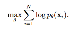
然而,上面的这个公式要求 p θ ( x ) p_{\theta}(x) pθ(x)是一个规则化的PDF,而这对于计算 p θ ( x ) p_{\theta}(x) pθ(x)提出了挑战:
我们必须计算归一化常数 Z θ Z_{\theta} Zθ,对于任何一般情况下的 f θ ( x ) f_{\theta}(\bf{x}) fθ(x),这是一个典型的难以处理的量
所以,为了使得maximum likelihood training的训练变得可行,likelihood-based models通过如下2种方式,而这2种方式,尤其是FLOW-based模型,会使得计算量极具增加:
-
限制模型结构(causal convolutions in autoregressive models, invertible networks in normalizing flow models)来使得 Z θ = 1 Z_{\theta}=1 Zθ=1
-
近似规则化常数(variational inference in VAEs, or MCMC sampling used in contrastive divergence)
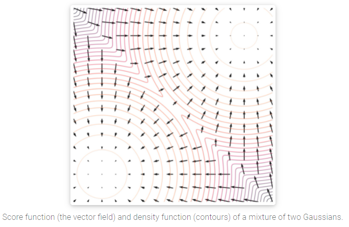
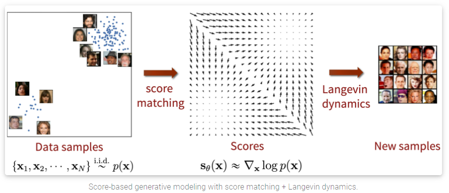
而score-based模型则是通过构造一个score function而非density function来避开处理这个规则化常数的问题。对一个分布 P ( x ) P(x) P(x), 其score function定义为:
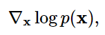
使用这种score function的模型我们就统称为score-based model, 用 s θ ( x ) s_{\theta}(\bf{x}) sθ(x)来表示,这种模型的目标是在无需考虑规则化常数项的情况下,使得 s θ ( x ) ≈ ∇ x l o g p ( x ) s_{\theta}(\bf{x}) \approx \nabla_{x} log p(x) sθ(x)≈∇xlogp(x)。以 p θ ( x ) = e − f θ ( x ) Z θ p_{\theta}(x)=\frac{e^{-f_{\theta}(\bf{x})}}{Z_{\theta}} pθ(x)=Zθe−fθ(x)为例进行展开,得到如下结果:
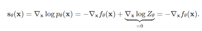
可以看出, s θ ( x ) s_{\theta}(\bf{x}) sθ(x)和normalizing constant Z θ Z_{\theta} Zθ相互独立。这个性质可以保证我们可以扩展生成模型的类别,并无需像之前的likelihood类方法那样,通过设计复杂的结构来使得 Z θ Z_{\theta} Zθ易于处理(tractable).
Parameterizing probability density functions(pdfs). No matter how you change the model family and parameters, it has to be normalized (area under the curve (AUC) must integrate to one).
Parameterizing score functions. No need to worry about normalization.
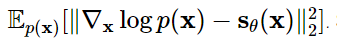
同likelihood类方法类似,我们可以通过最小化the Fisher divergence between the model and the data distributions来训练得到一个score-based models:
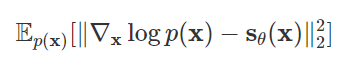
直觉上来说,Fisher divergence (Fisher散度)是计算ground-truth数据和score-based模型的 l 2 l_2 l2距离的平方。但是由于不知道数据得分 ∇ x l o g p ( x ) \nabla_{x} log p(x) ∇xlogp(x), 我们没法直接优化Fisher divergence. 幸运的是,现存了一系列称之为score matching的方法[12,13,14],这种方式可以在不知道ground-truth data score的情况下,minimize Fisher divergence.
score matching的objectives(目标)可以在给定数据上通过SGD(随机梯度下降)的方式估计得到。类比于 log-likelihood objective 在训练likelihood-based models的情况。
Score matching objectives can directly be estimated on a dataset and optimized with stochastic gradient descent, analogous to the log-likelihood objective for training likelihood-based models (with known normalizing constants
我们可以训练一个score-based模型来优化score-matching objective, 而不需要对抗学习!
此外,使用score matching objective给了我们在模型结构设计的灵活性。Fisher Divergence不需要 s θ ( x ) s_{\theta}(\bf{x}) sθ(x)是任意的规则化分布的实际得分函数(actual score function). 即: 无需像之前的方法那样,对 s θ ( x ) s_{\theta}(\bf{x}) sθ(x)有一个较强的假设! 在使用中,score-based model的唯一要求是
score-based model should be a vector-valued function with the same input and output dimensionality, which is easy to satisfy in practice.
本节内容,我们可以通过建模score function来模拟/代表一种分布,这种模型的构建是通过使用score matching技术来得到的。
3. Langevin dynamics (郎之万动力学)
一旦我们训练得到一个 s θ ( x ) ≈ ∇ x l o g p ( x ) s_{\theta}(\bf{x}) \approx \nabla_{x} log p(x) sθ(x)≈∇xlogp(x),我们可以使用 Langevin dynamics[15,16]的方法来迭代式的进行数据采样。
Langevin dynamics仅通过使用score function ∇ x l o g p ( x ) \nabla_{x} log p(x) ∇xlogp(x)来对真实数据分布 P ( x ) P(x) P(x)进行MCMC(MCMC, 马尔科夫链蒙特卡洛(Markov Chain Monte Carlo)方法,是用于从复杂分布中获取随机样本的统计学算法)的采样。具体来说,它先从任意的先验的分布中 x 0 ∼ π ( x ) \bf{x}_{0} \sim \bf{\pi(x)} x0∼π(x), 初始化构造一个chain,然后按着下面公式所述的那样进行迭代:
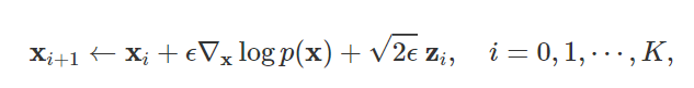
这里, z i ∼ N ( 0 , I ) \bf{z}_{i} \sim N(0, I) zi∼N(0,I), 当 ϵ \epsilon ϵ趋近于0且 K \bf{K} K趋近于无穷的时候,在常规条件下, x K \bf{x}_{K} xK近似于实际数据分布 P ( x ) P(x) P(x)的数据,两者的误差在 ϵ \epsilon ϵ足够小且 K \bf{K} K足够大的时候,可以忽略不计。这就说明,可以通过Langevin dynamics来采样得到我们希望得到的和原始数据分布一模一样的分布!
![[外链图片转存失败,源站可能有防盗链机制,建议将图片保存下来直接上传(img-oWZtpic9-1624072358558)(http://yang-song.github.io/assets/img/score/langevin.gif)]](https://img-blog.csdnimg.cn/20210619111256920.png)
4. 最基础的score-based模型以及其问题
截至目前,我们讨论了如何用score matching来优化训练一个score-based模型,并使用Langevin dynamics的方法去做数据采样。然而,这种最朴素的方式在实践中通常不太work,本节的内容主要聚焦在这些问题(secret pitfalls)上面。
目前的版本,由于在score matching中的一些问题,导致出现了较为明显的失败情况,而这些问题,前人的文章并没有仔细的探究。
一个核心的挑战(key challenge)是估计出来的score function在低维空间非常不准确。我们之前提到,score-based模型是通过最小化F真实数据和模型输出的Fisher divergence进行的
但是,由于true data score function and score-based model 的 l 2 l_2 l2 误差由数据分布 P ( x ) P(x) P(x)决定,而真实数据分布在低维空间被极大的扭曲和扰动,因此无法代表真实的数据分布了。这种情况导致了低于平均水平(subpar)的结果,如下图所示:
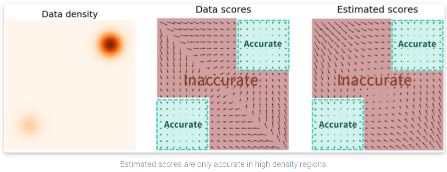
当使用 Langevin dynamics进行数据采样时,我们的初始样本极易出现在low density区域而非高维空间。因此,基于一个不准确的score-based模型进行采样,会让Langevin dynamics的采样过程derail(出轨),无法生成高质量的,能够代表真实数据分布的数据!
5. multiple noise perturbation后的score-based模型
如第4部分所说,我们如何绕过在低维空间/低密度区域中,score估计的准确性问题呢? 我们的思路是对数据点进行扰动,并让我们的模型在这种noisy data上面进行训练。
当噪声的幅度足够大时,它可以填充低数据密度区域,以提高估计分数的准确性。具体的,下图就是我们使用额外的高斯噪声对混合高斯模型进行扰动的结果:
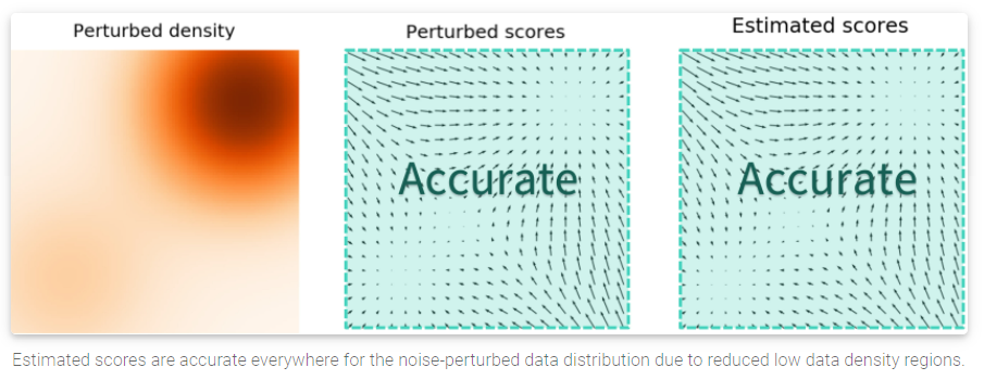
但是这引发了另一个问题:我们该怎样选择适合的噪声幅度来进行扰动呢?更大的噪声可以明显的覆盖更多的低密度区域,提升score estimation结果。但是它会极大的损害数据本身,并使其偏离原始的数据分布。
而微小的噪声扰动则无法cover我们所希望覆盖的低密度区域(low density regions),即使其对原始数据的分布没有做出很大的改变。
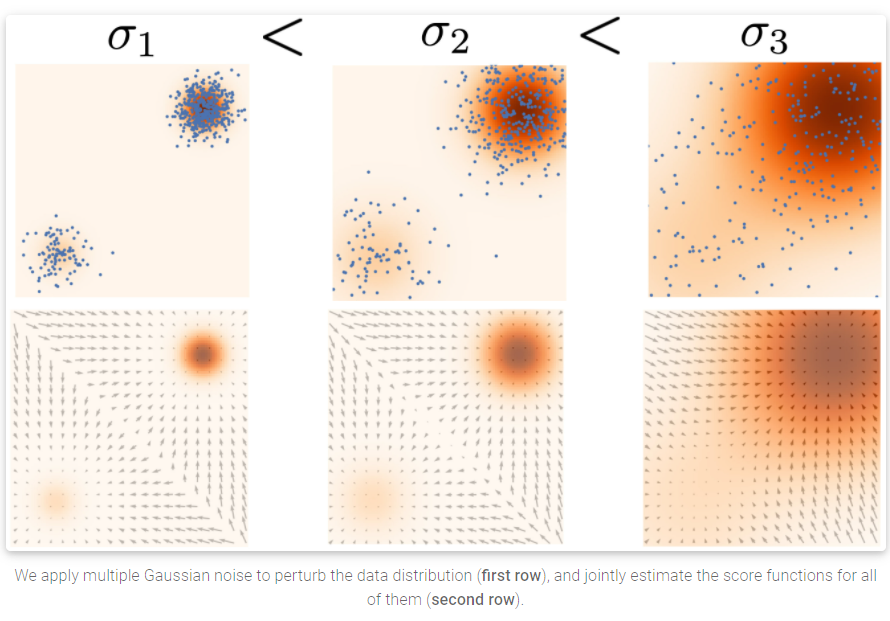
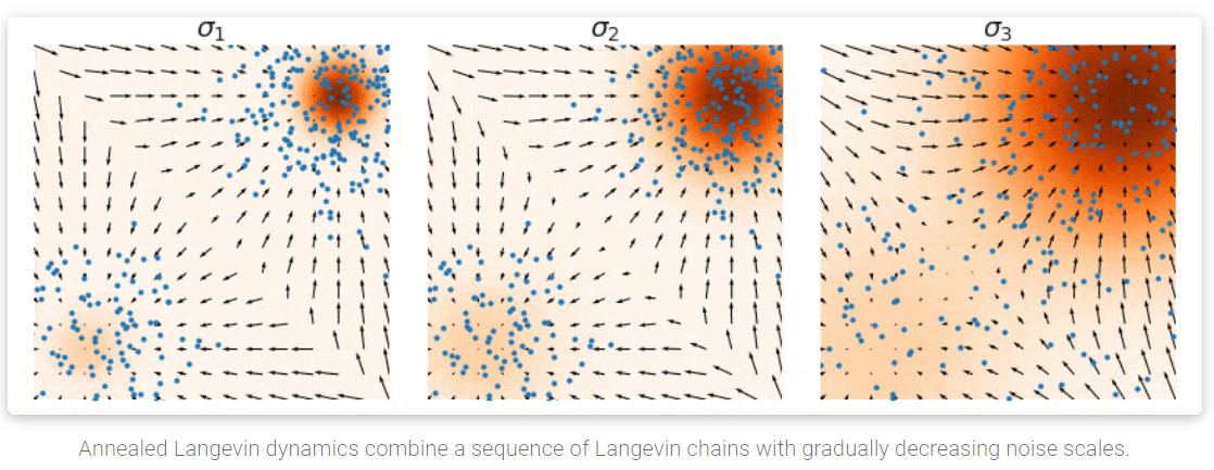
为了达到最佳的效果,宋博士提出了同时使用多尺度的噪声干扰[8, 9]。假设我们总是用均值为零(mean zero)的各向同性高斯噪声(isotropic Gaussian noise)来干扰数据, 假设有 L L L个扰动信号,标准差从小到大排列: σ 1 < σ 2 < . . . < σ L \sigma_1 < \sigma_2 < … < \sigma_L σ1<σ2<...<σL, 首先,用每个扰动信号去扰动数据 P ( x ) P(x) P(x):
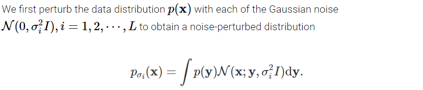
注意,我们可以通过对 x ∼ P ( x ) x \sim P(x) x∼P(x)采样,并计算 x + σ i z \bf{x} + \sigma_i \bf{z} x+σiz来得到被第i个噪声扰动后的数据,其中 z ∼ N ( 0 , I ) \bf{z} \sim N(0, I) z∼N(0,I)。
第二步,我们通过训练Noise Conditional Score-Based Model s θ ( x , i ) s_{\theta}(\bf{x, i}) sθ(x,i),对每个被噪声扰动的分布的score function进行估计: ∇ x l o g p σ i ( x ) \nabla_{\bf{x}} log p_{\sigma_i}(\bf{x}) ∇xlogpσi(x),以使得:

那么接下来就很符合直觉了,训练的目标 s θ ( x , i ) s_{\theta}(\bf{x, i}) sθ(x,i)是不同噪声尺度 L L L的加权结果。具体的,我们使用如下的目标函数:
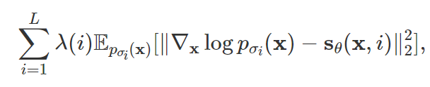
这里唯一需要注意的是权重 λ ( i ) \lambda(i) λ(i)的取值, 在宋博士的论文中,让 λ ( i ) = σ i 2 \lambda(i)=\sigma_i^{2} λ(i)=σi2. 这个目标函数可以使用score matching技术进行优化,就跟优化最朴素的score based model s θ ( x ) s_{\theta}(\bf{x}) sθ(x)一样。
在得到noise-conditional 的score-based模型 s θ ( x , i ) s_{\theta}(\bf{x, i}) sθ(x,i)后,我们就可以使用Langevin Dynamics来进行采样了. i = L , L − 1 , . . . , 1 i=L, L-1, …, 1 i=L,L−1,...,1. 这种方法称之为退火Langevin Dynamics算法(Annealed Langevin Dynamics, 在[8]的算法1中定义), 之所以称之为退火,可以理解为噪声的幅度是逐渐缩小的。
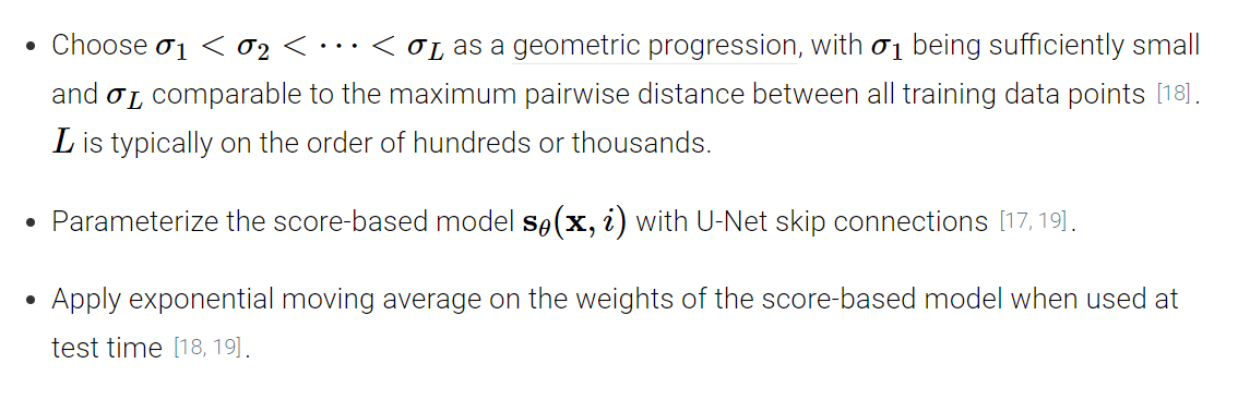
下面是一些用于训练一个score-based生成模型with multiple noise scale的实用的建议:
- 噪声的等级由低到高最好要有成百上千个级别.
- U-Net结构来设计模型.
- 在测试阶段,使用EMA.

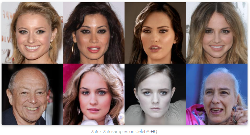
Annealed Langevin dynamics for the Noise Conditional Score Network (NCSN) model (from ref.
[17]) trained on CelebA . We can start from complete noise, modify images according to the scores, and generate nice samples. The method achieved state-of-the-art Inception score on CIFAR-10 at its time.
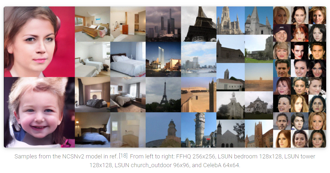
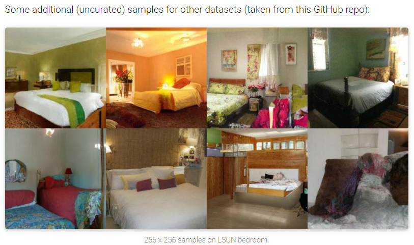
使用上面的说明,我们可以生成和GAN类似的高质量的图像样本,如下所示:
6. Score-based generative modeling with stochastic differential equations (SDEs)
根据前面的讨论,我们知道在score-based生成模型训练中,加入多层次、尺度的噪声是成功的关键因素。现在,当我们想把噪声的数量扩展到infinity(无限)的时候,我们可以基于score-based生成模型构造迄今为止最强大的框架。这不仅可以生成更高质量的样本,而且可以用精确地log-likelihood来优化模型,并加快采样速度,使得学习的特征具有更好的,更加独立的表征,并且可以用于编辑(inverse problem solving).
宋博士提供了Google Colab的版本来完成一个step-by-step的MNIST模型的训练。同样的,对更复杂的任务有更复杂的模型。
6.1 使用SDE(随机微分方程)来扰动数据
当噪声的规模和尺度趋近于无穷时,我们本质上是在用逐渐增加的噪声来干扰数据。在这种情况下,噪声干扰过程是一个随时间连续的随机过程(continuous-time stochastic process)
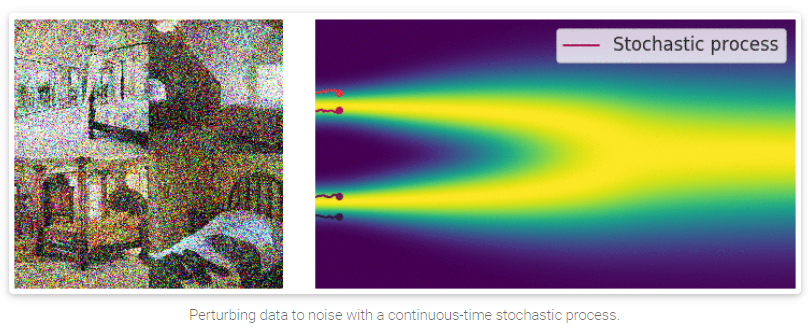
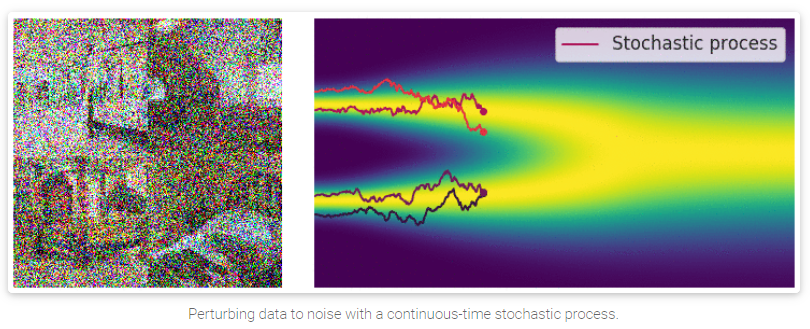
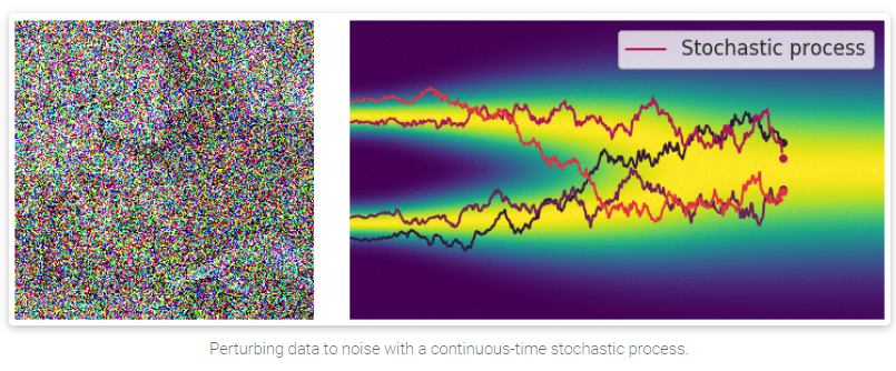
GIF图具体看
[1], 这里可以看到,随着随机过程的加深,原图的信息被大量的隐藏起来。
那么,怎么能够用更加精确地方式来表示这种随机过程呢?随机的随机过程(以扩散过程为例)是SDEs(随机微分方程)的解。一般地,SDE具有如下的形式:
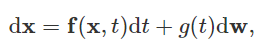
f ( x , t ) : R d → R d \mathbf{f}(\mathbf{x}, t) : \mathbb{R}^d \rightarrow \mathbb{R}^d f(x,t):Rd→Rd代表的是飘移系数(drift coefficient), g ( t ) ∈ R g(t) \in \mathbb{R} g(t)∈R表示的是扩散系数, w \mathbf{w} w则表示为标准的布朗运动, d w \mathrm{d}\mathbf{w} dw可以视为无穷小的白噪声(infinitesimal white noise)。这个随机微分方程的解是一组连续的随机变量 { x ( t ) } t ∈ [ 0 , T ] \{\mathbf{x}(t)\}_{t \in [0, T]} {
x(t)}t∈[0,T],这些随机变量描述在t时刻的轨迹。
用 p t ( x ) p_t(\mathbf{x}) pt(x)来表示 x ( t ) \mathbf{x}(t) x(t)的边缘概率密度函数。这里的 t ∈ [ 0 , T ] t \in [0, T] t∈[0,T]可以类比为不同尺度下的噪声 i = 1 , 2 , . . . , L i = 1, 2, …, L i=1,2,...,L; p t ( x ) p_t(\mathbf{x}) pt(x)可以类比为 p σ i ( x ) p_{\sigma_i}(\mathbf{x}) pσi(x)。这里, p 0 ( x ) = p ( x ) p_0(\mathbf{x}) = p(\mathbf{x}) p0(x)=p(x)代表了本来的数据分布(没有噪声干扰的情况)。
在用随机过程的方法对 p ( x ) p(\mathbf{x}) p(x)干扰了足够长的时间 T T T后, p T ( x ) p_T(\mathbf{x}) pT(x)已经变成了一个简单的随机噪声分布,我们将其表示为一个prior distribution(先验分布), 相似地,这可以类比为有限扰动尺度下的 p σ L ( x ) p_{\sigma_L}(\mathbf{x}) pσL(x)。
我们知道,对数据进行扰动的方式非常多,选择SDEs的方式进行扰动也没啥特别的。如下式这种SDE,是使用均值为0,方差指数增长的高斯噪声对数据进行干扰,这同之前的 N ( 0 , σ 1 2 I ) , N ( 0 , σ 2 2 I ) , . . . , N ( 0 , σ L 2 I ) N(0, \sigma_1^2I), N(0, \sigma_2^2I), …, N(0, \sigma_L^2I) N(0,σ12I),N(0,σ22I),...,N(0,σL2I)类似。
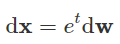
因此,SDE的过程应该被视为模型的超参数,如 { σ 1 , σ 2 , . . . , σ L } \{\sigma_1, \sigma_2, … , \sigma_L\} {
σ1,σ2,...,σL}。对图像生成任务,我们提供了3种比较适合这个领域的SDE。
6.2 Reverse SDE用于生成样本
之前我们提到的annealed Langevin dynamics(退火郎之万动力学算法), 其方式是按顺序从每个噪声干扰的分布中,使用Langevin dynamics的方式进行采样。对于我们的这种SDE的方式(无穷噪声),也可以使用类似的方式来进行。
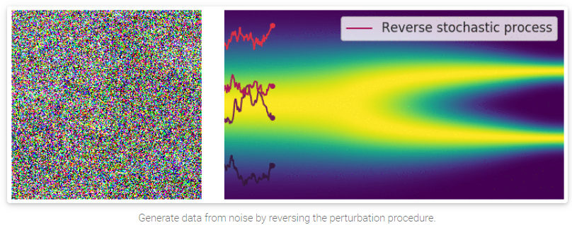
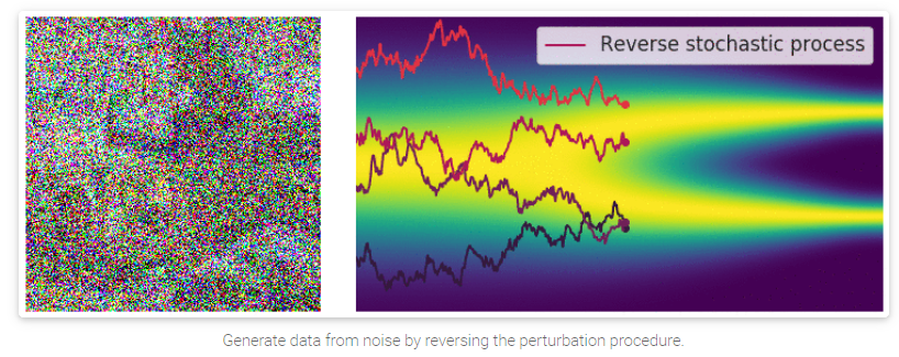
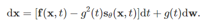
需要注意的是,SDE是可逆的,有其对应的Inverse SDE, 有着明确的close-form solution:
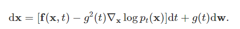
这里, d t \mathrm{d}t dt表示负的无穷小时间步,由于SDE需要被逆向求解(从时间 t = T t=T t=T到时间 t = 0 t=0 t=0), 那么我们需要对 ∇ x l o g p t ( x ) \nabla_{\mathbf{x}}log p_t(\mathbf{x}) ∇xlogpt(x)进行估计,而这与 p t ( x ) p_t(\mathbf{x}) pt(x)的score function是一样的。
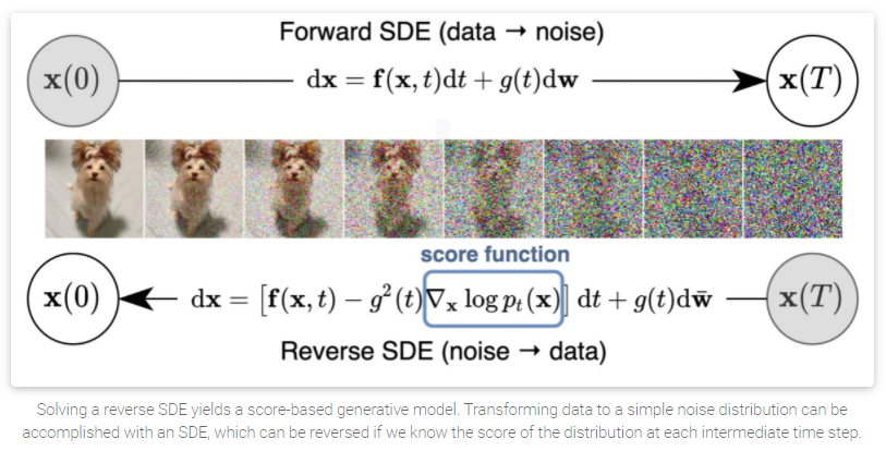
6.3 Estimating the reverse SDE with score-based models and score matching
如6.2所述,我们需要估计 ∇ x l o g p t ( x ) \nabla_{\mathbf{x}}log p_t(\mathbf{x}) ∇xlogpt(x)来逆向求解,得到被噪声干扰前的图像、语音等信息。那么,为了估计 ∇ x l o g p t ( x ) \nabla_{\mathbf{x}}log p_t(\mathbf{x}) ∇xlogpt(x),我们提出一种 Time-Dependent Score-Based Model s θ ( x , t ) \mathbf{s}_{\theta}(\mathbf{x}, t) sθ(x,t), 从而使得 s θ ( x , t ) ≈ ∇ x l o g p t ( x ) \mathbf{s}_{\theta}(\mathbf{x}, t) \approx \nabla_{\mathbf{x}}log p_t(\mathbf{x}) sθ(x,t)≈∇xlogpt(x)。同样,这可以和noise-conditional score-based model s θ ( x , i ) \mathbf{s}_{\theta}(\mathbf{x}, i) sθ(x,i)进行类比。
我们对于 s θ ( x , t ) \mathbf{s}_{\theta}(\mathbf{x}, t) sθ(x,t)的训练目标很直接,就是一个连续的Fisher散度的Mixture:
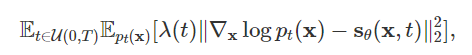
这里 u ( 0 , T ) u(0, T) u(0,T)表示在 [ 0 , T ] [0, T] [0,T]的均匀分布, λ > 0 : R → R \lambda > 0: \mathbb{R} \rightarrow \mathbb{R} λ>0:R→R表示为不同时间下的噪声权重,是正的。
我们用如下的方程(当 λ ( t ) = g 2 ( t ) \lambda(t) = g^2(t) λ(t)=g2(t))来表示 λ ( t ) \lambda(t) λ(t):
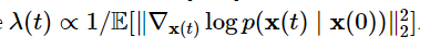
这里,Fisher散度和KL散度产生了一些奇妙的联系:

这里, p t \mathtt{p}_t pt和 q t \mathtt{q}_t qt分别代表 x t \mathbf{x}_{t} xt的分布( x ( 0 ) ∼ p 0 \mathbf{x}(0) \sim \mathtt{p}_0 x(0)∼p0和 x ( 0 ) ∼ q 0 \mathbf{x}(0) \sim \mathtt{q}_0 x(0)∼q0)。
由于KL散度和Fisher散度的特殊联系以及KL散度和最大似然估计的等价性,
我们将 λ ( t ) = g 2 ( t ) \lambda(t) = g^2(t) λ(t)=g2(t)称为似然权重函数likelihood weighting function。
同之前讲的那样, 我们的目标函数: 混合Fisher散度(mixture of Fisher divergence)能够通过score matching方法进行高效的优化,如denoising score matching[17]以及sliced score matching[14]。
当我们的score-based模型训练完毕后,我们可以将其插入reverse SDE过程中,用于数据的采样过程。
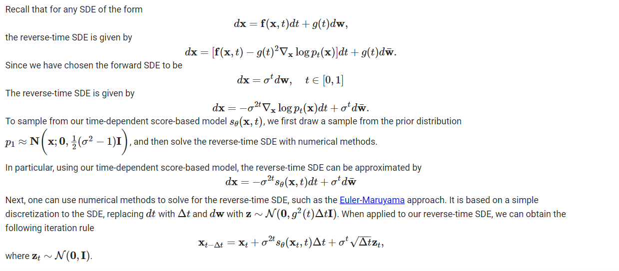
6.4 How to solve the reverse SDE
通过数值SDE求解器,我们可以估计reverse SDE,我们可以模拟reverse随机过程来用于生成样本。最简单的数值SDE求解器也许是Euler-Maruyama方法。当将其应用到我们的SDE中,Euler-Maruyama方法使用有限的时间步和小的高斯噪声去离散SDE。具体来讲,就是其选择了small, negative的时间步,进行初始化,然后按照下列方式进行迭代优化直到 t ≈ 0 t \approx 0 t≈0:
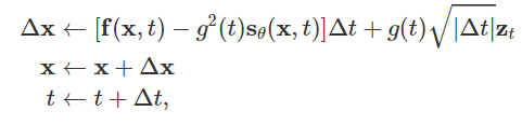
这里 z t ∼ N ( 0 , I ) \mathbf{z}_t \sim N(0, I) zt∼N(0,I), Euler-Maruyama 方法和Langevin dynamics方法的性质很相似: “They both update x \mathbf{x} x by following score functions perturbed with Gaussian noise”.
除了Euler-Maruyama方法外,还有一些可以直接用于求解SDE逆过程的方法: Milstein 方法[18]以及stochastic Runge-Kutta 方法[19], 在宋博士最新的ICLR2021的论文中,提出了一种新的reverse diffusion solver来近似Euler-Maruyama方法,这种方法更适合解决reverse-time的SDE。
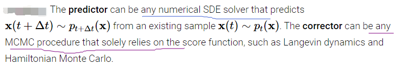
对我们的reverse SDE,有2类特殊的性质可以使得我们进行更为灵活的采样:
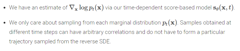
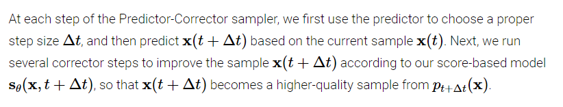
基于上面的2个性质,我们可以使用马尔科夫链蒙特卡洛方法去fine-tune通过数值SDE solver得到的轨迹(trajectories)。宋博士提出了Predictor-Corrector samplers.
实际对照MNIST代码,我发现采样过程如下所示 \sigma^{2t}实际上就是 g ( t ) 2 g(t)^2 g(t)2, 以500次迭代为例进行分析,我们可以将其和公式一一对应起来,得到扰动前的结果。
num_steps =  500#@param {'type':'integer'}
def Euler_Maruyama_sampler(score_model,
                           marginal_prob_std,
                           diffusion_coeff,
                           batch_size=64,
                           num_steps=num_steps,
                           device='cuda',
                           eps=1e-3):
  """Generate samples from score-based models with the Euler-Maruyama solver. Args: score_model: A PyTorch model that represents the time-dependent score-based model. marginal_prob_std: A function that gives the standard deviation of the perturbation kernel. diffusion_coeff: A function that gives the diffusion coefficient of the SDE. batch_size: The number of samplers to generate by calling this function once. num_steps: The number of sampling steps. Equivalent to the number of discretized time steps. device: 'cuda' for running on GPUs, and 'cpu' for running on CPUs. eps: The smallest time step for numerical stability. Returns: Samples. """
  t = torch.ones(batch_size, device=device)
  init_x = torch.randn(batch_size, 1, 28, 28, device=device) \
    * marginal_prob_std(t)[:, None, None, None]
  time_steps = torch.linspace(1., eps, num_steps, device=device)
  step_size = time_steps[0] - time_steps[1]
  x = init_x
  with torch.no_grad():
    for time_step in tqdm.notebook.tqdm(time_steps):
      batch_time_step = torch.ones(batch_size, device=device) * time_step
      g = diffusion_coeff(batch_time_step) # g(t) 扩散系数.
      mean_x = x + (g**2)[:, None, None, None] * score_model(x, batch_time_step) * step_size
      x = mean_x + torch.sqrt(step_size) * g[:, None, None, None] * torch.randn_like(x)
  # Do not include any noise in the last sampling step.
  return mean_x
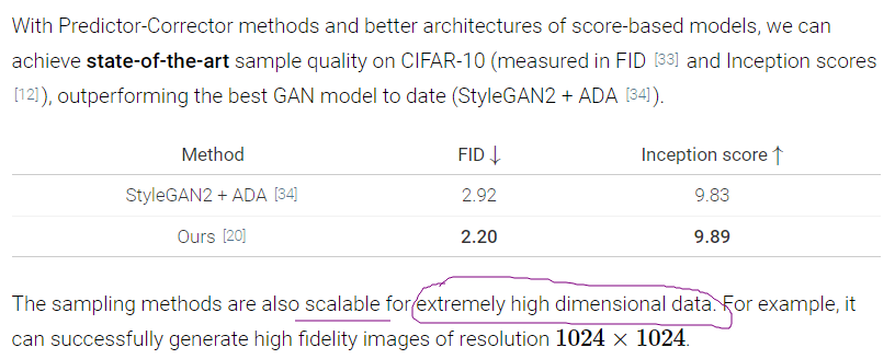
随着Predictor-Corrector方法来优化采样过程,以及更好的score-based模型架构的提出,宋博士的算法在CIFAR10上达到了SOTA效果,并且比StyleGAN2取得的效果还要惊人!
参考资料
[1]: Generative Modeling by Estimating Gradients of the Data Distribution: 宋飏-20210505
[2]: The neural autoregressive distribution estimator
[3]: NICE: Non-linear independent components estimation
[4]: A Tutorial on Energy-Based Learning
[5]: Auto-encoding variational bayes
[6]: Unrolled Generative Adversarial Networks
[7] A kernelized Stein discrepancy for goodness-of-fit tests
[8] Generative Modeling by Estimating Gradients of the Data Distribution
[9] Improved Techniques for Training Score-Based Generative Models
[10] Learning Gradient Fields for Shape Generation
[11] 最大似然估计
[12] Estimation of non-normalized statistical models by score matching
[13] A connection between score matching and denoising autoencoders
[14] Sliced score matching: A scalable approach to density and score estimation
[15] Correlation functions and computer simulations, 1981, G. Parisi.
[16] Representations of knowledge in complex systems, 1994, U. Grenander, M.I. Miller.
[17] A connection between score matching and denoising autoencoders
[18] Milstein method
[19] Runge–Kutta method (SDE)
发布者:全栈程序员-用户IM,转载请注明出处:https://javaforall.cn/169751.html原文链接:https://javaforall.cn
【正版授权,激活自己账号】: Jetbrains全家桶Ide使用,1年售后保障,每天仅需1毛
【官方授权 正版激活】: 官方授权 正版激活 支持Jetbrains家族下所有IDE 使用个人JB账号...
