大家好，又见面了，我是你们的朋友全栈君。

一、什么是自动编码器？

        自编码器是开发无监督学习模型的主要方式之一。但什么是自动编码器？

        简而言之，自动编码器通过接收数据、压缩和编码数据，然后从编码表示中重构数据来进行操作。对模型进行训练，直到损失最小化并且尽可能接近地再现数据。通过这个过程，自动编码器可以学习数据的重要特征。

        自动编码器是由多个层组成的神经网络。自动编码器的定义方面是输入层包含与输出层一样多的信息。输入层和输出层具有完全相同数量的单元的原因是自动编码器旨在复制输入数据。然后分析数据并以无监督方式重建数据后输出数据副本。

        通过自动编码器的数据不仅仅是从输入直接映射到输出。自动编码器包含三个组件：压缩数据的编码（输入）部分、处理压缩数据（或瓶颈）的组件和解码器（输出）部分。当数据被输入自动编码器时，它会被编码，然后压缩到更小的尺寸。然后对网络进行编码/压缩数据的训练，并输出该数据的重建。

        神经网络学习了输入数据的“本质”或最重要的特征，这是自动编码器的核心价值。训练完网络后，训练好的模型就可以合成相似的数据，并添加或减去某些目标特征。例如，您可以在加了噪声的图像上训练自动编码器，然后使用经过训练的模型从图像中去除噪声。

        自编码器的应用包括：异常检测、数据去噪（例如图像、音频）、图像着色、图像修复、信息检索等、降维等。

二、自动编码器的架构

        自动编码器基本上可以分为三个不同的组件：编码器、瓶颈和解码器。

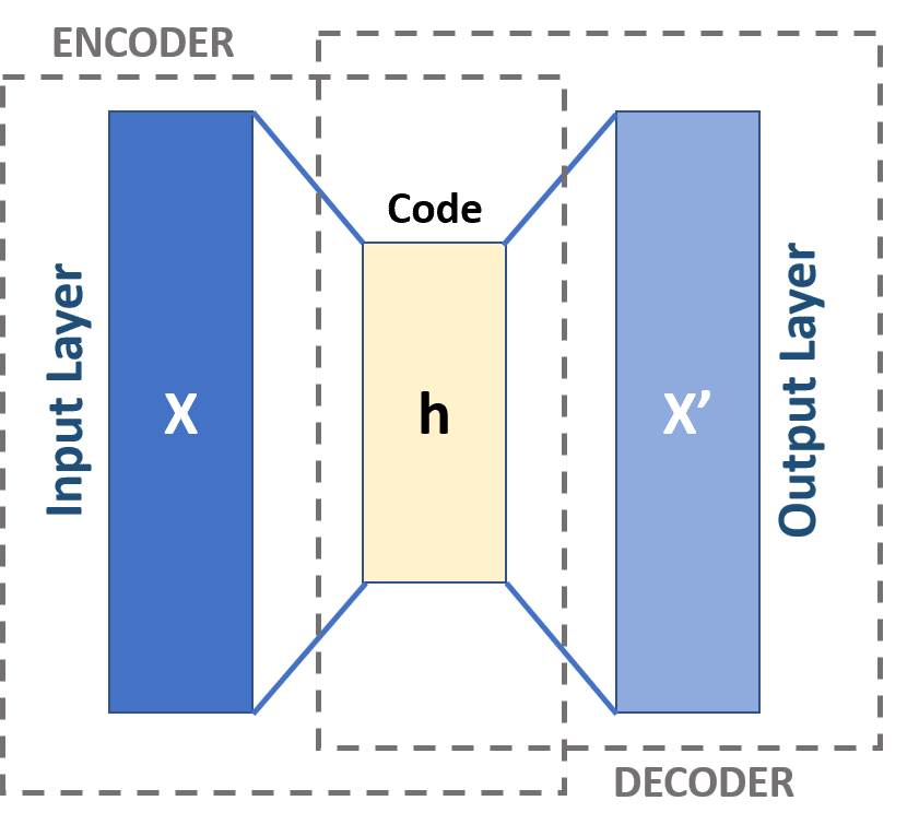
        编码器：编码器是一个前馈、全连接的神经网络，它将输入压缩为潜在空间表示，并将输入图像编码为降维的压缩表示。压缩后的图像是原始图像的变形版本。

        code：网络的这一部分包含输入解码器的简化表示。

        解码器：解码器和编码器一样也是一个前馈网络，结构与编码器相似。该网络负责将输入从代码中重建回原始维度。

        首先，输入通过编码器进行压缩并存储在称为code的层中，然后解码器从代码中解压缩原始输入。自编码器的主要目标是获得与输入相同的输出。

        通常情况下解码器架构是编码器的镜像，但也不是绝对的。唯一的要求是输入和输出的维度必须相同。

三、自动编码器的类型

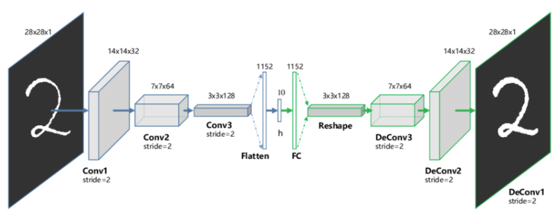
1、卷积自动编码器

        卷积自动编码器是通用的特征提取器。卷积自编码器是采用卷积层代替全连接层，原理和自编码器一样，对输入的象征进行降采样以提供较小维度潜在表示，并强制自编码器学习象征的压缩版本。

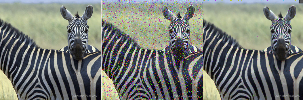
 2、去噪自动编码器

        这种类型的自动编码器适用于部分损坏的输入，并训练以恢复原始未失真的图像。如上所述，这种方法是限制网络简单复制输入的有效方法。

        目标是网络将能够复制图像的原始版本。通过将损坏的数据与原始数据进行比较，网络可以了解数据的哪些特征最重要，哪些特征不重要/损坏。换句话说，为了让模型对损坏的图像进行去噪，它必须提取图像数据的重要特征。

3、收缩自动编码器

        收缩自动编码器的目标是降低表示对训练输入数据的敏感性。 为了实现这一点，在自动编码器试图最小化的损失函数中添加一个正则化项或惩罚项。

        收缩自动编码器通常仅作为其他几种自动编码器节点存在。去噪自动编码器使重建函数抵抗输入的小但有限大小的扰动，而收缩自动编码器使特征提取函数抵抗输入的无穷小扰动。

4、变分自动编码器

        Variational Autoencoders，这种类型的自动编码器对潜在变量的分布做出了假设，并在训练过程中使用了随机梯度变分贝叶斯估计器。

        训练时，编码器为输入图像的不同特征创建潜在分布。

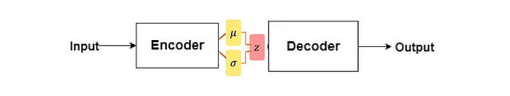
        本质上，该模型学习了训练图像的共同特征，并为它们分配了它们发生的概率。然后可以使用概率分布对图像进行逆向工程，生成与原始训练图像相似的新图像。 

        这种类型的自动编码器可以像GAN一样生成新图像。由于 VAE 在生成行为方面比GAN更加灵活和可定制，因此它们适用于任何类型的艺术生成。

四、自动编码器与PCA有何不同？

        PCA 和自动编码器是降低特征空间维数的两种流行方法。

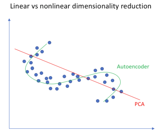
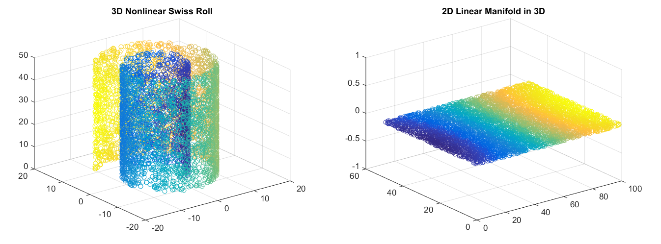
         PCA 从根本上说是一种线性变换，但自动编码器可以描述复杂的非线性过程。如果我们要构建一个线性网络（即在每一层不使用非线性激活函数），我们将观察到与 PCA 中相似的降维。

        PCA 试图发现描述原始数据的低维超平面，而自动编码器能够学习非线性流形（流形简单地定义为连续的、不相交的表面）。

         与自动编码器相比，PCA 的计算速度更快且成本更低。但由于参数数量多，自编码器容易过拟合。

五、自编码器与GAN有何不同？

        1、两者都是生成模型。AE试图找到以特定输入（更高维度）为条件的数据的低维表示，而GAN 试图创建足以概括以鉴别器为条件的真实数据分布的表示。

        2、虽然它们都属于无监督学习的范畴，但它们是解决问题的不同方法。

        GAN 是一种生成模型——它应该学习生成数据集的新样本。

        变分自动编码器是生成模型，但普通的自动编码器只是重建它们的输入，不能生成真实的新样本。

https://www.quora.com/What-is-the-difference-between-Generative-Adversarial-Networks-and-Autoencodershttps://www.quora.com/What-is-the-difference-between-Generative-Adversarial-Networks-and-Autoencoders

六、实例1：去噪自动编码器

1、概述

        去噪自动编码器的一个应用的例子是预处理图像以提高光学字符识别 (OCR) 算法的准确性。如果您以前应用过OCR，就会知道一丁点错误的噪声（例如，打印机墨水污迹、扫描过程中的图像质量差等）都会严重影响OCR识别的效果。使用去噪自编码器，可以自动对图像进行预处理，提高质量，从而提高OCR识别算法的准确性。

        我们这里故意向MNIST训练图像添加噪声。目的是使我们的自动编码器能够有效地从输入图像中去除噪声。

2、参考代码

        创建autoencoder_for_denoising.py文件，插入以下代码。

# import the necessary packages
from tensorflow.keras.layers import BatchNormalization
from tensorflow.keras.layers import Conv2D
from tensorflow.keras.layers import Conv2DTranspose
from tensorflow.keras.layers import LeakyReLU
from tensorflow.keras.layers import Activation
from tensorflow.keras.layers import Flatten
from tensorflow.keras.layers import Dense
from tensorflow.keras.layers import Reshape
from tensorflow.keras.layers import Input
from tensorflow.keras.models import Model
from tensorflow.keras import backend as K
import numpy as np

class ConvAutoencoder:
	@staticmethod
	def build(width, height, depth, filters=(32, 64), latentDim=16):
		# initialize the input shape to be "channels last" along with
		# the channels dimension itself
		# channels dimension itself
		inputShape = (height, width, depth)
		chanDim = -1
		# define the input to the encoder
		inputs = Input(shape=inputShape)
		x = inputs

		# loop over the number of filters
		for f in filters:
			# apply a CONV => RELU => BN operation
			x = Conv2D(f, (3, 3), strides=2, padding="same")(x)
			x = LeakyReLU(alpha=0.2)(x)
			x = BatchNormalization(axis=chanDim)(x)
		# flatten the network and then construct our latent vector
		volumeSize = K.int_shape(x)
		x = Flatten()(x)
		latent = Dense(latentDim)(x)
		# build the encoder model
		encoder = Model(inputs, latent, name="encoder")

		# start building the decoder model which will accept the
		# output of the encoder as its inputs
		latentInputs = Input(shape=(latentDim,))
		x = Dense(np.prod(volumeSize[1:]))(latentInputs)
		x = Reshape((volumeSize[1], volumeSize[2], volumeSize[3]))(x)
		# loop over our number of filters again, but this time in
		# reverse order
		for f in filters[::-1]:
			# apply a CONV_TRANSPOSE => RELU => BN operation
			x = Conv2DTranspose(f, (3, 3), strides=2, padding="same")(x)
			x = LeakyReLU(alpha=0.2)(x)
			x = BatchNormalization(axis=chanDim)(x)
		# apply a single CONV_TRANSPOSE layer used to recover the
		# original depth of the image
		x = Conv2DTranspose(depth, (3, 3), padding="same")(x)
		outputs = Activation("sigmoid")(x)
		# build the decoder model
		decoder = Model(latentInputs, outputs, name="decoder")
		# our autoencoder is the encoder + decoder
		autoencoder = Model(inputs, decoder(encoder(inputs)), name="autoencoder")
		# return a 3-tuple of the encoder, decoder, and autoencoder
		return (encoder, decoder, autoencoder)


# set the matplotlib backend so figures can be saved in the background
import matplotlib
matplotlib.use("Agg")
# import the necessary packages
from tensorflow.keras.optimizers import Adam
from tensorflow.keras.datasets import mnist
import matplotlib.pyplot as plt
import numpy as np
import argparse
import cv2
# construct the argument parse and parse the arguments
ap = argparse.ArgumentParser()
ap.add_argument("-s", "--samples", type=int, default=8, help="# number of samples to visualize when decoding")
ap.add_argument("-o", "--output", type=str, default="output.png", help="path to output visualization file")
ap.add_argument("-p", "--plot", type=str, default="plot.png", help="path to output plot file")
args = vars(ap.parse_args())

# initialize the number of epochs to train for and batch size
EPOCHS = 25
BS = 32
# load the MNIST dataset
print("[INFO] loading MNIST dataset...")
((trainX, _), (testX, _)) = mnist.load_data()
# add a channel dimension to every image in the dataset, then scale
# the pixel intensities to the range [0, 1]
trainX = np.expand_dims(trainX, axis=-1)
testX = np.expand_dims(testX, axis=-1)
trainX = trainX.astype("float32") / 255.0
testX = testX.astype("float32") / 255.0

# sample noise from a random normal distribution centered at 0.5 (since
# our images lie in the range [0, 1]) and a standard deviation of 0.5
trainNoise = np.random.normal(loc=0.5, scale=0.5, size=trainX.shape)
testNoise = np.random.normal(loc=0.5, scale=0.5, size=testX.shape)
trainXNoisy = np.clip(trainX + trainNoise, 0, 1)
testXNoisy = np.clip(testX + testNoise, 0, 1)

# construct our convolutional autoencoder
print("[INFO] building autoencoder...")
(encoder, decoder, autoencoder) = ConvAutoencoder.build(28, 28, 1)
opt = Adam(lr=1e-3)
autoencoder.compile(loss="mse", optimizer=opt)
# train the convolutional autoencoder
H = autoencoder.fit(trainXNoisy, trainX, validation_data=(testXNoisy, testX), epochs=EPOCHS, batch_size=BS)
# construct a plot that plots and saves the training history
N = np.arange(0, EPOCHS)
plt.style.use("ggplot")
plt.figure()
plt.plot(N, H.history["loss"], label="train_loss")
plt.plot(N, H.history["val_loss"], label="val_loss")
plt.title("Training Loss and Accuracy")
plt.xlabel("Epoch #")
plt.ylabel("Loss/Accuracy")
plt.legend(loc="lower left")
plt.savefig(args["plot"])


# use the convolutional autoencoder to make predictions on the
# testing images, then initialize our list of output images
print("[INFO] making predictions...")
decoded = autoencoder.predict(testXNoisy)
outputs = None
# loop over our number of output samples
for i in range(0, args["samples"]):
	# grab the original image and reconstructed image
	original = (testXNoisy[i] * 255).astype("uint8")
	recon = (decoded[i] * 255).astype("uint8")
	# stack the original and reconstructed image side-by-side
	output = np.hstack([original, recon])
	# if the outputs array is empty, initialize it as the current
	# side-by-side image display
	if outputs is None:
		outputs = output
	# otherwise, vertically stack the outputs
	else:
		outputs = np.vstack([outputs, output])
# save the outputs image to disk
cv2.imwrite(args["output"], outputs)

        然后输入以下命令进行训练。

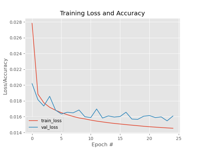
python train_denoising_autoencoder.py --output output_denoising.png --plot plot_denoising.png

3、训练结果

        经过25epoch的训练结果。

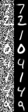
         对应的去噪结果图，左边是添加噪声的原始MNIST数字，而右边是去噪自动编码器的输出——可以看到去噪自动编码器能够在消除噪音的同时从图像中恢复原始信号。