大家好，又见面了，我是你们的朋友全栈君。

机械狗

写在前面

可能要写很长很久，可能一年吧

计划

目前我打算先做模拟，然后在模拟环境中设计控制器，全部调得很完美后再开始搭。平台选择是这样的：

目前对狗的器官是这么设想的：

1 搭建模拟环境

1.1先模拟条简单的狗腿 （two-link)

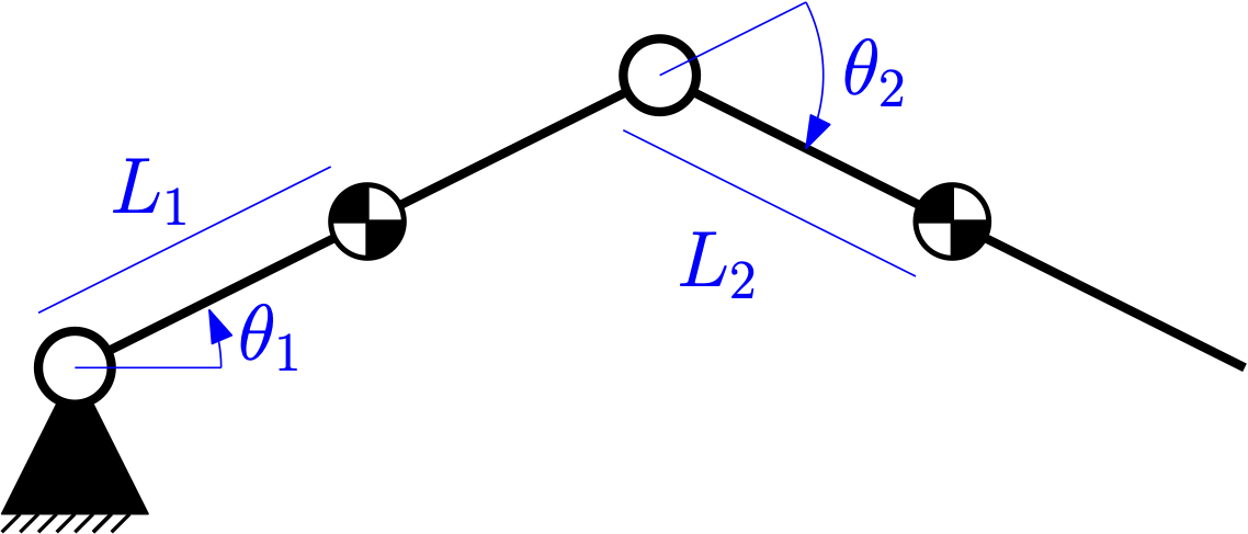
为了方便起见，先就忽略转动惯量了。这个其实应该没什么大事，毕竟我要造的玩具狗腿摆得又不会很快。这里第一个关节代表腿根部，两杆子的末端（end-effector,EE)是狗脚。

1.1.1 Forward Kinematics

这边我用matlab里symbolic math 来推导所有的kinematics.
这里x2 y2 是 EE 的位置。

sympref('AbbreviateOutput', false); 
% prevent symbolic abbreviations
syms L1 L2 theta1 theta2
x1 = 2*L1*cos(theta1);
y1 = 2*L1*sin(theta1);
x2 = x1 + 2*L2*cos(theta1+theta2);
y2 = y1 + 2*L2*sin(theta1+theta2);
Xee= [x2;
      y2] %end effector position

Matlab output: (直接复制symbolic 的latex code,然后最外面加四美元号）
$$\left(\begin{array}{c}2L_2\cos \left({\theta }_1+{\theta }_2\right)+2L_1\cos \left({\theta }_1\right)\\ 2L_2\sin \left({\theta }_1+{\theta }_2\right)+2L_1\sin \left({\theta }_1\right)\end{array}\right)$$
最后把这个解析解变成一个可以输入数值的方程：

fk_two_link_func = matlabFunction(Xee)

1.1.2 Inverse Kinematics

Inverse Kinematics 就是给EE的位置算出达到这个位置时关节需要的角度。注意，kinematics完全不考虑外力啊什么的。
算这个inverse kinematics 有两种算法：
一种是手推，具体推法可以参考这个视频：

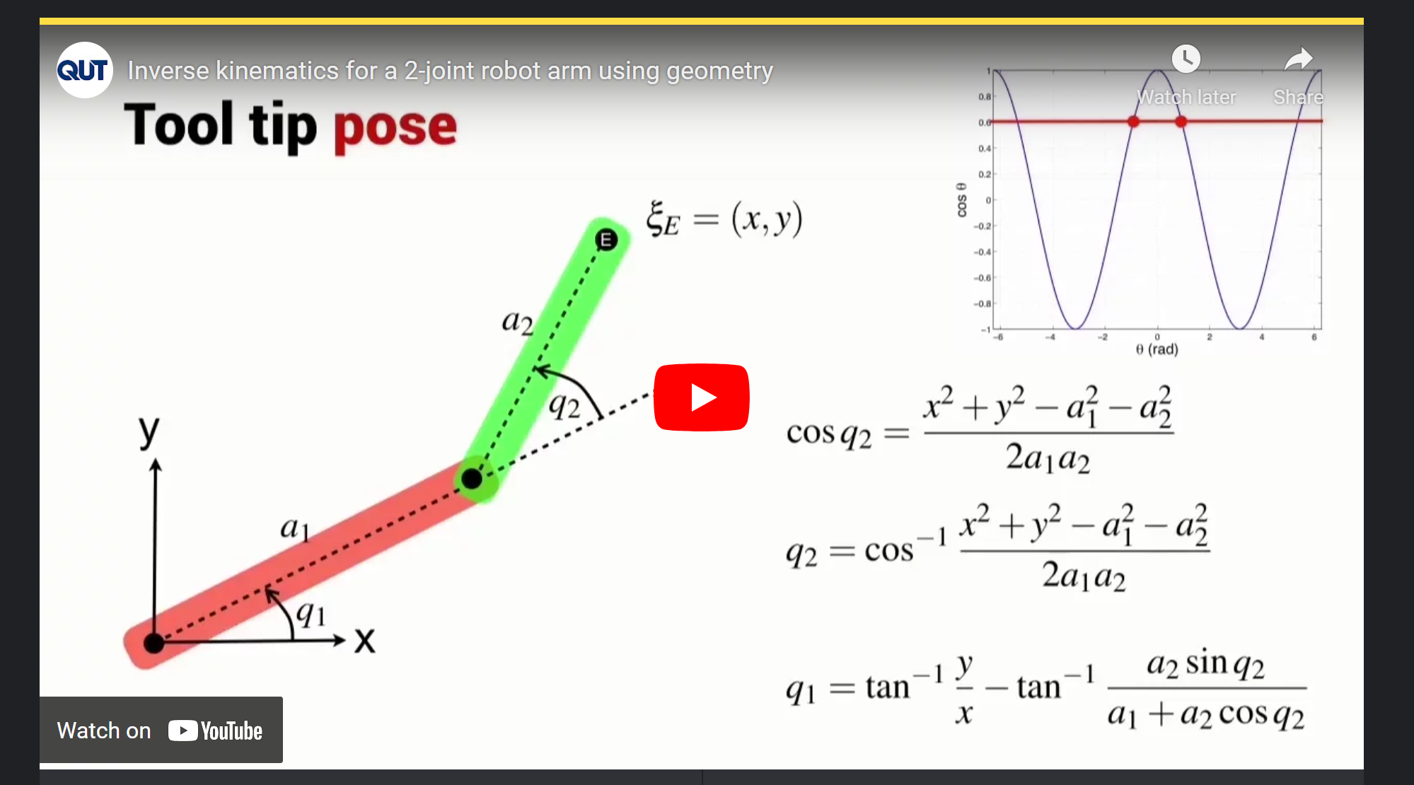
但这玩意有个问题，只能在第一象限用。本人对三角函数啥的一直没很彻底的 悟 。 所以也不知道为啥只能在第一象限用。

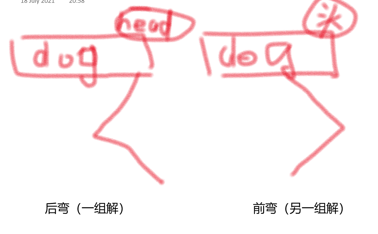
第二种是直接用symbolic math 自动推。好处是四个象限都能用，而且不可能出错。最重要的它能给出所有的解：选择适合的解能帮助我们实现狗腿是向前弯还是向后弯。

第三种是用matlab里的robotic toolbox，但我现在还没试过。

第二种方法代码如下，xt yt 是目标点的坐标：

sympref('AbbreviateOutput', false); 
% prevent symbolic abbreviations
syms L1 L2 theta1 theta2
x1 = 2*L1*cos(theta1);
y1 = 2*L1*sin(theta1);
x2 = x1 + 2*L2*cos(theta1+theta2);
y2 = y1 + 2*L2*sin(theta1+theta2);
Xee= [x2;
      y2]; %end effector position
      
syms xt yt
eq_ik_twolink_RHS = [xt;
                     yt];
Theta_twolink = [theta1;
                 theta2];
S_ik_twolink = solve(Xee==eq_ik_twolink_RHS,Theta_twolink);
ik_two_link = [S_ik_twolink.theta1;
               S_ik_twolink.theta2];
ik_two_link = simplify(ik_two_link)

Output:
$$\left(\begin{array}{c}2\mathrm{a}\mathrm{t}\mathrm{a}\mathrm{n}\left(\frac{4L_1\mathrm{y}\mathrm{t}+\sqrt{-16{L_1}^4+32{L_1}^2{L_2}^2+8{L_1}^2{\mathrm{x}\mathrm{t}}^2+8{L_1}^2{\mathrm{y}\mathrm{t}}^2-16{L_2}^4+8{L_2}^2{\mathrm{x}\mathrm{t}}^2+8{L_2}^2{\mathrm{y}\mathrm{t}}^2-{\mathrm{x}\mathrm{t}}^4-2{\mathrm{x}\mathrm{t}}^2{\mathrm{y}\mathrm{t}}^2-{\mathrm{y}\mathrm{t}}^4}}{4{L_1}^2+4L_1\mathrm{x}\mathrm{t}-4{L_2}^2+{\mathrm{x}\mathrm{t}}^2+{\mathrm{y}\mathrm{t}}^2}\right)\\ 2\mathrm{a}\mathrm{t}\mathrm{a}\mathrm{n}\left(\frac{4L_1\mathrm{y}\mathrm{t}-\sqrt{-16{L_1}^4+32{L_1}^2{L_2}^2+8{L_1}^2{\mathrm{x}\mathrm{t}}^2+8{L_1}^2{\mathrm{y}\mathrm{t}}^2-16{L_2}^4+8{L_2}^2{\mathrm{x}\mathrm{t}}^2+8{L_2}^2{\mathrm{y}\mathrm{t}}^2-{\mathrm{x}\mathrm{t}}^4-2{\mathrm{x}\mathrm{t}}^2{\mathrm{y}\mathrm{t}}^2-{\mathrm{y}\mathrm{t}}^4}}{4{L_1}^2+4L_1\mathrm{x}\mathrm{t}-4{L_2}^2+{\mathrm{x}\mathrm{t}}^2+{\mathrm{y}\mathrm{t}}^2}\right)\\ -2\mathrm{a}\mathrm{t}\mathrm{a}\mathrm{n}\left(\frac{\sqrt{\left(-4{L_1}^2+8L_1{L}_2-4{L_2}^2+{\mathrm{x}\mathrm{t}}^2+{\mathrm{y}\mathrm{t}}^2\right)\left(4{L_1}^2+8L_1{L}_2+4{L_2}^2-{\mathrm{x}\mathrm{t}}^2-{\mathrm{y}\mathrm{t}}^2\right)}}{-4{L_1}^2+8L_1{L}_2-4{L_2}^2+{\mathrm{x}\mathrm{t}}^2+{\mathrm{y}\mathrm{t}}^2}\right)\\ 2\mathrm{a}\mathrm{t}\mathrm{a}\mathrm{n}\left(\frac{\sqrt{\left(-4{L_1}^2+8L_1{L}_2-4{L_2}^2+{\mathrm{x}\mathrm{t}}^2+{\mathrm{y}\mathrm{t}}^2\right)\left(4{L_1}^2+8L_1{L}_2+4{L_2}^2-{\mathrm{x}\mathrm{t}}^2-{\mathrm{y}\mathrm{t}}^2\right)}}{-4{L_1}^2+8L_1{L}_2-4{L_2}^2+{\mathrm{x}\mathrm{t}}^2+{\mathrm{y}\mathrm{t}}^2}\right)\end{array}\right)$$
注意，这里一共有四个输出，分别依次对应theta1的两个解，theta2的两个解。这样形成的两组解就对应那张前弯后弯图里情况。

把这个解也变成方程，

ik_two_link_func = matlabFunction(ik_two_link)

然后我们验证下：给定一个目标点的xy坐标，然后用inverse kinematics 算出角度。再把这角度带到forward kinematics 里，得到的答案应该和最开始的目标点重合。

L_twolink = [0.5 0.5] %meters, L1 L2;
Xtest = [1.1 1];        %meters, xtarget ytarget
ang_from_ik_two_link = ik_two_link_func( L_twolink(1),L_twolink(1),...
                                         Xtest(1),Xtest(2) )
%Note there are four outputs. They correspond to: theta1_solution_1, theta1_solution_2, theta2_solution_1 and theta2_solution_2.
posi_from_fk_two_link = fk_two_link_func ( L_twolink(1),L_twolink(1),...
                                           ang_from_ik_two_link(1), ...
                                           ang_from_ik_two_link(3) )

接下来，我们到SIMSCAPE 里验证下：（以后可能会放出源码）

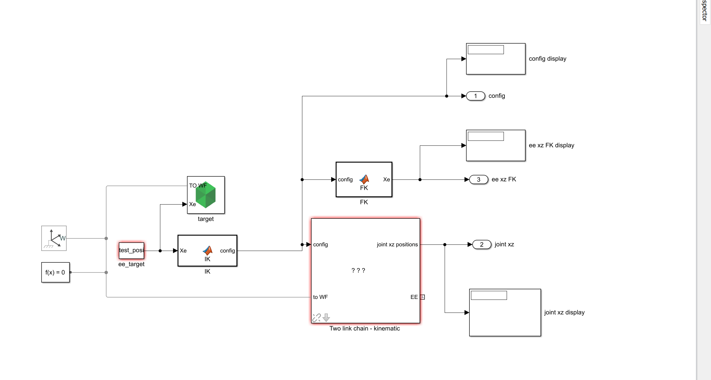
open_system('twolink_inverse_kinematics_w2')

% Set target postion and link length using polar cooridinate
% link one length = 2*L1
rho_two_link = [1;
                1]; %L1 L2 = 0.5m
rho = rho_two_link;
max_length_two_link = rho_two_link(1) + rho_two_link(2);
test_ang = 5.7;
test_length = 1.5;
test_posi = [cos(test_ang)*test_length;
             sin(test_ang)*test_length]
sim('twolink_inverse_kinematics_w2');

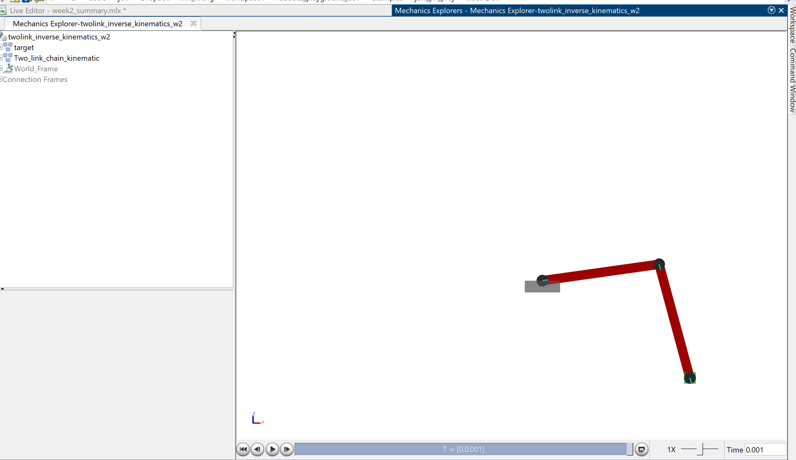
绿色的方块是目标点，可以看到EE完全到了目标点了。

1.1.3 Forward Dynamics

Dynamics 就要开始考虑力啦。这里我们会用拉格朗日法来算出动力学模型（是运动学还是动力学啊，有点分不清）。Again, 还是用symbolic math来自动推导 （symbolic 算lagragian 真的太爽啦啦啦啦）。

先定义下symbolic variable, 还是根据这张图来

clear all;
close all;
clc;
sympref('AbbreviateOutput', false); % prevent symbolic abbreviations

syms theta1 theta2 ...
     theta_dot_1 theta_dot_2 ...
     theta_ddot_1 theta_ddot_2 ...
     L1 L2 m1 m2 ...
     t g 

然后开始算lagrangian啦！注意，和之前不同的是，x1y1和x2y2代表了两个质点的位置，而不是之前kinematics推导中节点的位置

%Find position of two point mass in terms of the generalised coordinate %theta1 and theta2.
x1 = L1*cos(theta1);
y1 = L1*sin(theta1);
x2 = 2*x1 + L2*cos(theta1+theta2);
y2 = 2*y1 + L2*sin(theta1+theta2);
[x1 x2;
 y1 y2]
%Find velocity of the two point mass
x1_dot = diff(x1,theta1)*theta_dot_1 + diff(x1,theta2)*theta_dot_2;
x2_dot = diff(x2,theta1)*theta_dot_1 + diff(x2,theta2)*theta_dot_2;
y1_dot = diff(y1,theta1)*theta_dot_1 + diff(y1,theta2)*theta_dot_2;
y2_dot = diff(y2,theta1)*theta_dot_1 + diff(y2,theta2)*theta_dot_2;
[x1_dot, x2_dot;
 y1_dot, y2_dot];
%Find T U and L 
T = 0.5*m1*(x1_dot^2+y1_dot^2) + ...
    0.5*m2*(x2_dot^2+y2_dot^2);
U = (m1*g*L1*sin(theta1) + ...
      m2*g*(2*L1*sin(theta1)+L2*sin(theta1+theta2) ));
L = T - U;

（好想吐槽CSDN的代码片，为什么就没有matlab的代码片啊啊。）
接下来用这个公式算运动学方程：
$$\frac{d}{dt}\left(\frac{\partial \mathbf{L}}{\partial {\dot{\theta }}_i}\right)-\left(\frac{\partial \mathbf{L}}{\partial {\theta }_i}\right)=\mathbf{F}$$
这边要稍微提下，这里的F是generalised force. 当generalised coordinate 是translational时，它的物理形式为力（单位N），相反，当generalised coordinate 是rotational时，（比如 角度），它的物理形式为力矩。这里，所有的机械臂/狗腿的推导都是基于generalised coordinate 为角度的形式，所以这里的F为力矩。

接下来开始用symbolic来算上面那公式里的每个项了。先暂时忽略F，因为可以最后再加上。还有这里要用不少chain rule, 建议拿只笔写写思考下。

dL_dtheta_dot_1 = diff(L,theta_dot_1);
dL_dtheta_dot_2 = diff(L,theta_dot_2);
dL_dtheta1 = diff(L,theta1);
dL_dtheta2 = diff(L,theta2);
d__dL_dtheta_dot_1__dt = diff(dL_dtheta_dot_1,theta1)*theta_dot_1 + ...
                         diff(dL_dtheta_dot_1,theta2)*theta_dot_2 + ...
                         diff(dL_dtheta_dot_1,theta_dot_1)*theta_ddot_1 + ...
                         diff(dL_dtheta_dot_1,theta_dot_2)*theta_ddot_2;
d__dL_dtheta_dot_2__dt = diff(dL_dtheta_dot_2,theta1)*theta_dot_1 + ...
                         diff(dL_dtheta_dot_2,theta2)*theta_dot_2 + ...
                         diff(dL_dtheta_dot_2,theta_dot_1)*theta_ddot_1 + ...
                         diff(dL_dtheta_dot_2,theta_dot_2)*theta_ddot_2;

d__dL_dtheta_dot__dt = [d__dL_dtheta_dot_1__dt;
                        d__dL_dtheta_dot_2__dt];
dL_dtheta = [dL_dtheta1;
             dL_dtheta2];

然后就解出来了

%Eq will the forward dynamics. We assume there is no generalised force here.
eq = simplify(d__dL_dtheta_dot__dt - dL_dtheta,'Steps',10);

对，就解完啦。贴下答案，但没啥可视性。
两个运动学方程：
$$\left(\begin{array}{c}{L_1}^2{m}_1{\ddot{\theta }}_1+4{L_1}^2{m}_2{\ddot{\theta }}_1+{L_2}^2{m}_2{\ddot{\theta }}_1+{L_2}^2{m}_2{\ddot{\theta }}_2+L_{2}g{m}_2\cos \left({\theta }_1+{\theta }_2\right)+L_{1}g{m}_1\cos \left({\theta }_1\right)+2L_{1}g{m}_2\cos \left({\theta }_1\right)-2L_1{L}_2{m}_2{{\dot{\theta }}_2}^2\sin \left({\theta }_2\right)+4L_1{L}_2{m}_2{\ddot{\theta }}_1\cos \left({\theta }_2\right)+2L_1{L}_2{m}_2{\ddot{\theta }}_2\cos \left({\theta }_2\right)-4L_1{L}_2{m}_2{\dot{\theta }}_1{\dot{\theta }}_2\sin \left({\theta }_2\right)\\ L_2{m}_2\left(2L_1\sin \left({\theta }_2\right){{\dot{\theta }}_1}^2+L_2{\ddot{\theta }}_1+L_2{\ddot{\theta }}_2+g\cos \left({\theta }_1+{\theta }_2\right)+2L_1{\ddot{\theta }}_1\cos \left({\theta }_2\right)\right)\end{array}\right)$$

1.1.4 Inverse Dynamics

然后呢，我们希望能找出个特thetaddot = balala的方程。 在忽略generalised force的情况下（在three-link时会考虑到，这里偷懒先略过），可以直接用matlab built-in的方程解出来。这就是inverse dynamics：

thetaddot_1 and thetaddot2: （通过”solve”来解的）

Theta_ddot = [theta_ddot_1;
              theta_ddot_2];
Theta_dot = [theta_dot_1;
             theta_dot_2];
Theta = [theta1;
         theta2];
Use solve function to get theta_ddot_1 and theta_ddot_2
This is inverse dynamics! 
S = solve(eq == [0;0],Theta_ddot); %solve to get theta1ddot and theta2ddot eq
[S.theta_ddot_1;
S.theta_ddot_2]

$$\left(\begin{array}{c}\frac{2g{m}_2\cos \left({\theta }_1+{\theta }_2\right)\cos \left({\theta }_2\right)-2g{m}_2\cos \left({\theta }_1\right)-g{m}_1\cos \left({\theta }_1\right)+2L_2{m}_2{{\dot{\theta }}_1}^2\sin \left({\theta }_2\right)+2L_2{m}_2{{\dot{\theta }}_2}^2\sin \left({\theta }_2\right)+4L_1{m}_2{{\dot{\theta }}_1}^2\cos \left({\theta }_2\right)\sin \left({\theta }_2\right)+4L_2{m}_2{\dot{\theta }}_1{\dot{\theta }}_2\sin \left({\theta }_2\right)}{-4L_1{m}_2{\cos \left({\theta }_2\right)}^2+L_1{m}_1+4L_1{m}_2}\\ -\frac{L_{1}g{m}_1\cos \left({\theta }_1+{\theta }_2\right)+4L_{1}g{m}_2\cos \left({\theta }_1+{\theta }_2\right)+2{L_1}^2{m}_1{{\dot{\theta }}_1}^2\sin \left({\theta }_2\right)+8{L_1}^2{m}_2{{\dot{\theta }}_1}^2\sin \left({\theta }_2\right)+2{L_2}^2{m}_2{{\dot{\theta }}_1}^2\sin \left({\theta }_2\right)+2{L_2}^2{m}_2{{\dot{\theta }}_2}^2\sin \left({\theta }_2\right)-L_{2}g{m}_1\cos \left({\theta }_1\right)-2L_{2}g{m}_2\cos \left({\theta }_1\right)+2L_{2}g{m}_2\cos \left({\theta }_1+{\theta }_2\right)\cos \left({\theta }_2\right)-2L_{1}g{m}_1\cos \left({\theta }_1\right)\cos \left({\theta }_2\right)-4L_{1}g{m}_2\cos \left({\theta }_1\right)\cos \left({\theta }_2\right)+4{L_2}^2{m}_2{\dot{\theta }}_1{\dot{\theta }}_2\sin \left({\theta }_2\right)+8L_1{L}_2{m}_2{{\dot{\theta }}_1}^2\cos \left({\theta }_2\right)\sin \left({\theta }_2\right)+4L_1{L}_2{m}_2{{\dot{\theta }}_2}^2\cos \left({\theta }_2\right)\sin \left({\theta }_2\right)+8L_1{L}_2{m}_2{\dot{\theta }}_1{\dot{\theta }}_2\cos \left({\theta }_2\right)\sin \left({\theta }_2\right)}{-4L_1{L}_2{m}_2{\cos \left({\theta }_2\right)}^2+L_1{L}_2{m}_1+4L_1{L}_2{m}_2}\end{array}\right)$$

未完

1.2 模拟个复杂点的狗腿 （three/four-link)

1.3 搭个全身

1.4 加入Contact modelling

1.5 合到一起

2 控制器设计

2.1 PD controll

2.2 Impedance/force control

2.2.1 Spring-damper system analgue

2.2.2 Implementaion