大家好,又见面了,我是你们的朋友全栈君。如果您正在找激活码,请点击查看最新教程,关注关注公众号 “全栈程序员社区” 获取激活教程,可能之前旧版本教程已经失效.最新Idea2022.1教程亲测有效,一键激活。
Jetbrains全家桶1年46,售后保障稳定
本文课件来自香港科技大学,我的母校,感谢ELEC
本节介绍RRT/RRT*的算法:
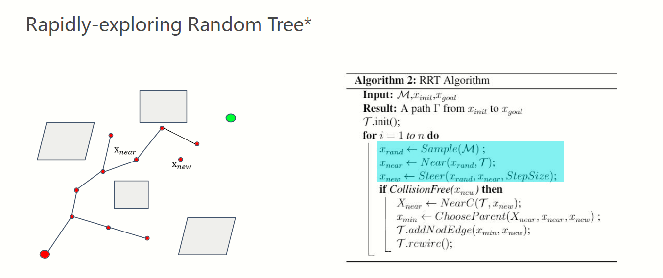
RRT的基本原理是:
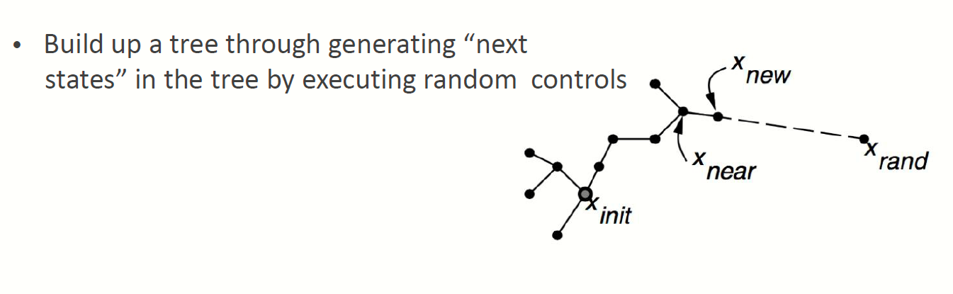

我们首先初始化我们的起点,接下来随机撒点,选出一个x_rand, 在x_near 和 x_rand之间选择一个x_new, 再在原有的已经存在的x中找到离这个点最近的点将这两个点连接起来,同时这个最近的点也会作为x_new的父节点。
RRT算法的伪代码如下:
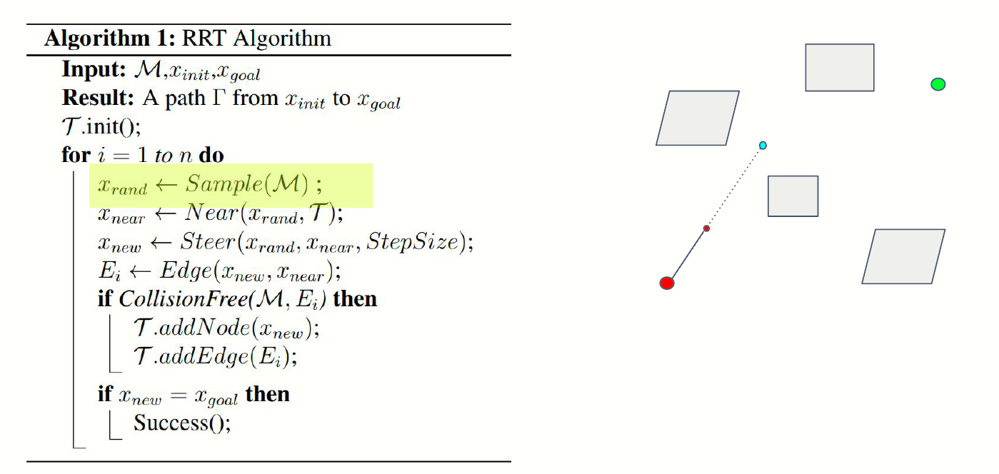
对照着图,再看一次:
首先我们随机生成一个点,x_rand
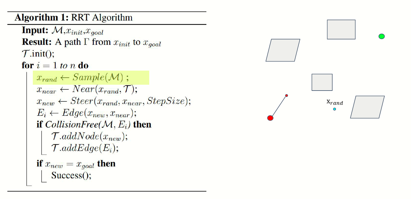
然后再tree上面找到最近点,作为x_near
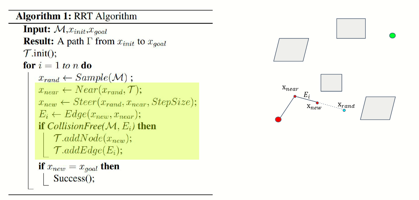
然后取两者中间的点作为x_new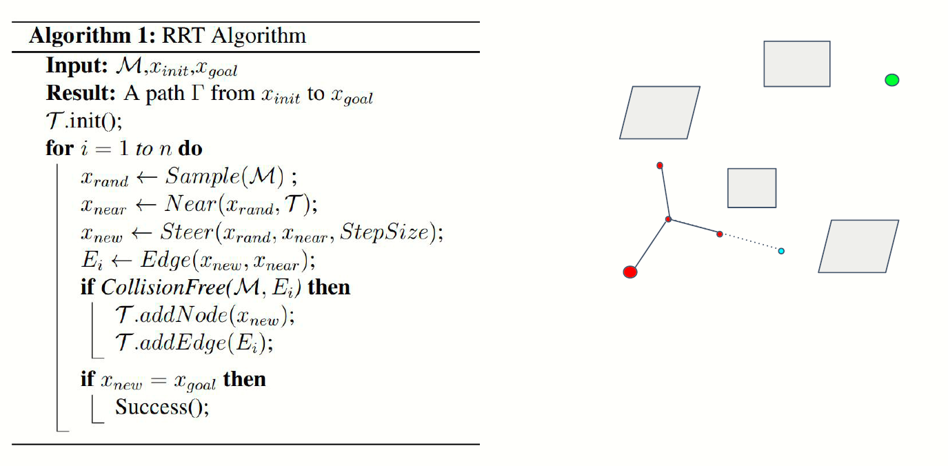
最后,还要做一次collision checking, 看看生成的点是不是和x_near 连接起来后会碰撞障碍物:
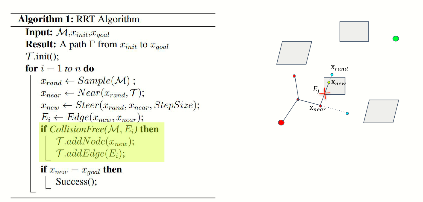
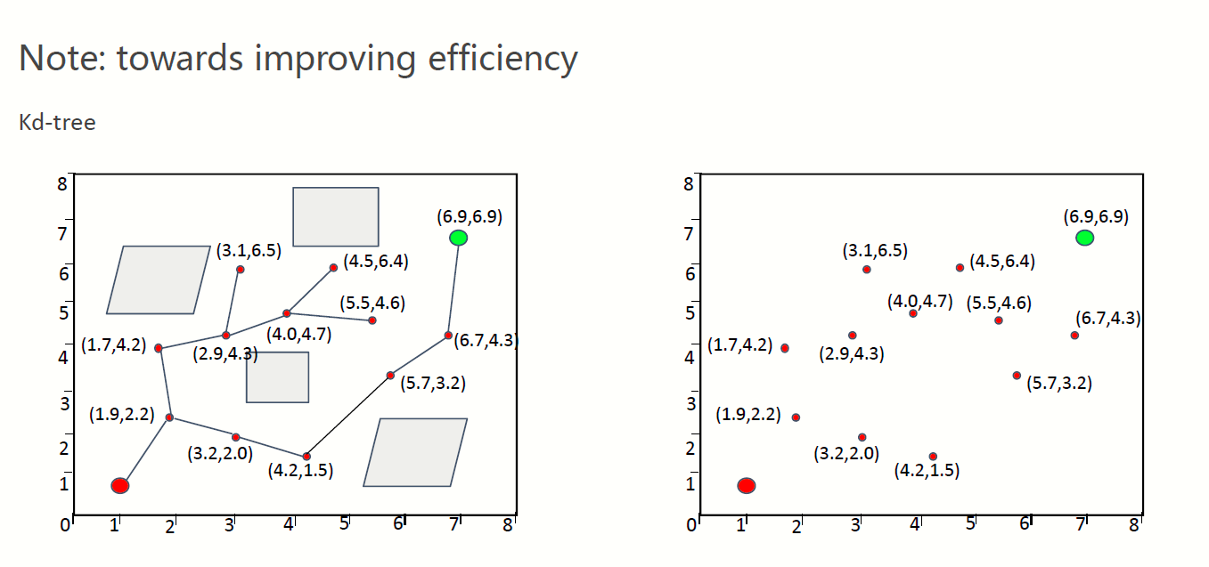
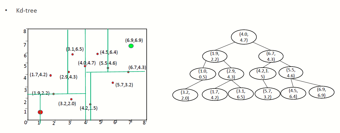
按照这个方法一直搜索,一直打到停止搜索的标准,比如x_new与终点的距离小于某个极小的epsilon。另外一个,在搜索最近的x_near的时候,我们可以使用KD tree来加速搜索:
具体看一下(https://blog.csdn.net/junshen1314/article/details/51121582)
接下来我们分析一下RRT的优缺点:

RRT比概率图方法更加有效,但是这依然不是个高效的搜索方法,并且获得的解也不是最优解。
接下里,我们有一些对RRT的优化方法:
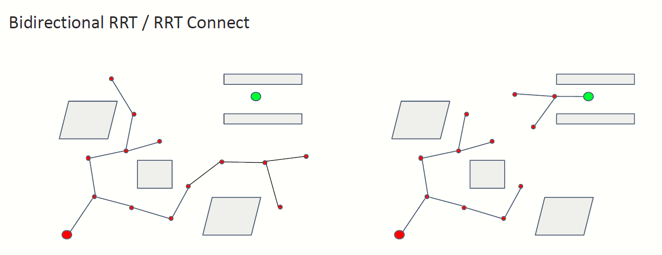
第一种方法就是双向RRT, 意思就是从起点和终点同时搜索,一直到两棵树交汇
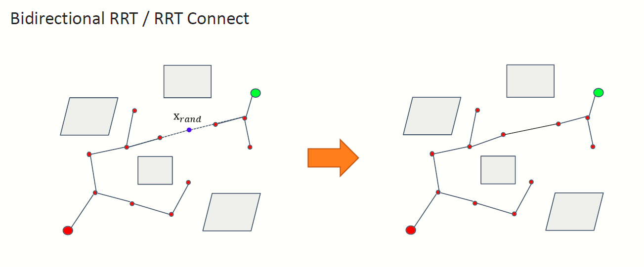
下图中可以看到,起点和终点同时生成树进行搜索。
第二种方法我们介绍RRT*
伪代码流程如下:
这个算法是在RRT基础上的改进,改进的地方是这个x_near 和 x_new不会直接连接起来,而是做一个优化处理,方式就是:
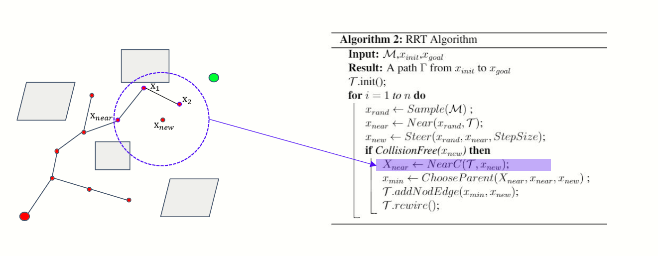
我们在x_near附近圈一个圆,将被圈在圈内的各个点与x_new的距离作对比:
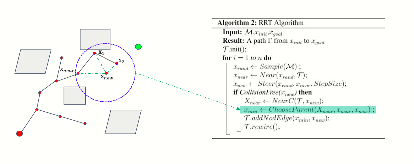
如果x_near 到 x_new的距离比通过x1,x2后再到x_new的距离低,就将x_near和x_new连接起来。

同时我们还要对比,从x_near出发,到x2的距离最短值:
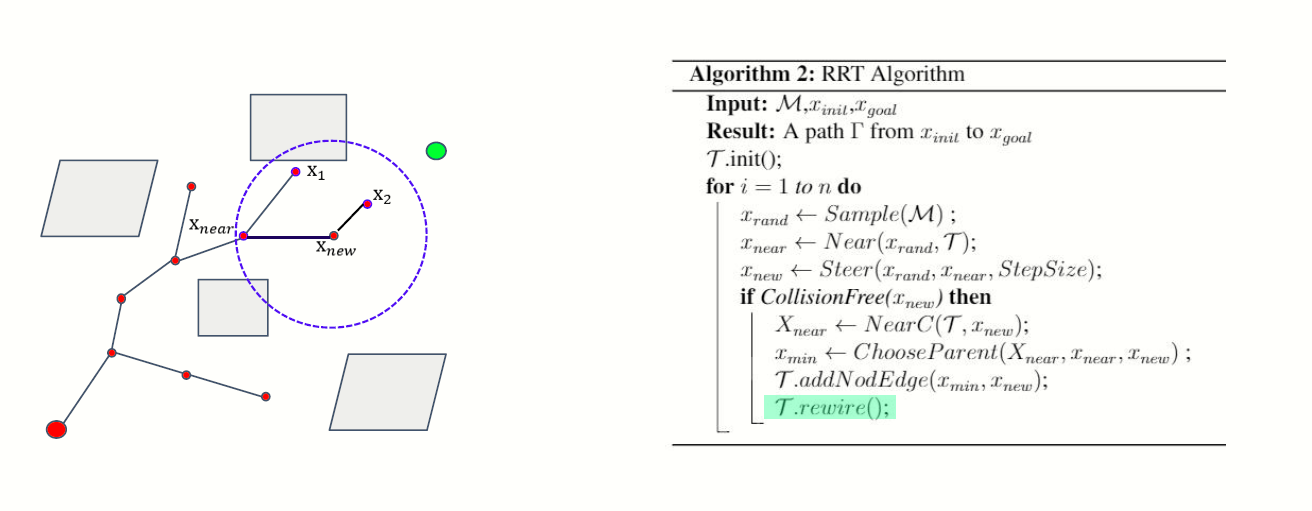
我们发现通过x_new之后到达x2的距离更短,所以就将x2的父节点更新为x_new. 这个步骤我们称之为rewire function.
相关视频演示参考:
https://www.youtube.com/watch?v=YKiQTJpPFkA
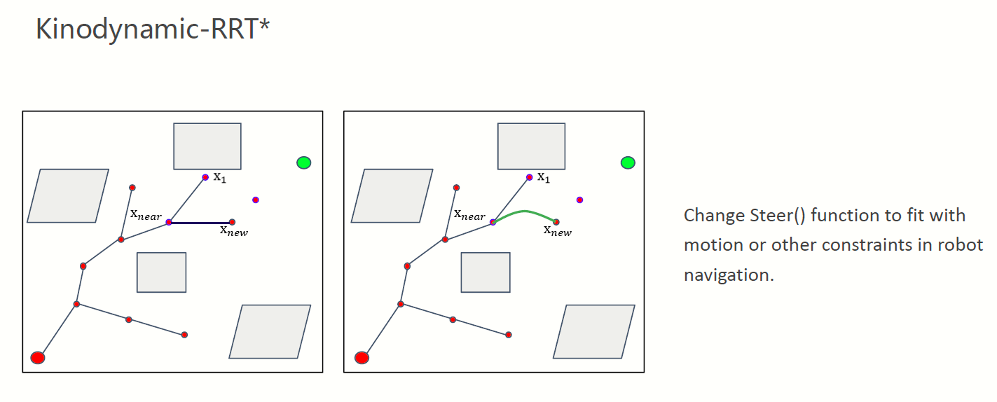
当然我们还有其他的优化,包括考虑动力学限制的优化:
接下来我们提供一系列源代码供读者进行测试:
首先提供2D RRT
%***************************************
%Author: Yuncheng JIANG
%***************************************
%% 流程初始化
clc;
clear all
close all
x_I=1; y_I=1;           % 设置初始点
x_G=700; y_G=700;       % 设置目标点
Thr=50;                 %设置目标点阈值
delta = 0.35 ;   % 设置扩展步长
iteration = 10000;
%% 建树初始化
T.v(1).x = x_I;         % T是我们要做的树,v是节点,这里先把起始点加入到T里面来
T.v(1).y = y_I;
T.v(1).xPrev = x_I;     % 起始节点的父节点仍然是其本身
T.v(1).yPrev = y_I;
T.v(1).dist=0;          %从父节点到该节点的距离,这里可取欧氏距离
T.v(1).indPrev = 0;     %
%% 开始构建树——作业部分
figure(1);
ImpRgb=imread('newmap.png');
Imp=rgb2gray(ImpRgb);
imshow(Imp)
xL=size(Imp,1);%地图x轴长度
yL=size(Imp,2);%地图y轴长度
hold on
plot(x_I, y_I, 'ro', 'MarkerSize',10, 'MarkerFaceColor','r');
plot(x_G, y_G, 'go', 'MarkerSize',10, 'MarkerFaceColor','g');% 绘制起点和目标点
count=1;
j =1;
for iter = 1:iteration
    iter
    x_rand(1) = rand(1)*800;
    x_rand(2) = rand(1)*800;
    x_rand = [x_rand(1),x_rand(2)];
    %Step 1: 在地图中随机采样一个点x_rand
    %提示:用(x_rand(1),x_rand(2))表示环境中采样点的坐标

    dist =zeros(length(T),1);

    for i =1: count
        dist(i) = (T.v(i).x- x_rand(1))^2 + (T.v(i).y - x_rand(2))^2;
        [value, location] = min(dist);
        x_near = [T.v(location).x,T.v(location).y];
    end
    %Step 2: 遍历树,从树中找到最近邻近点x_near
    %提示:x_near已经在树T里

    x_new=[x_near(1)+delta * (x_rand(1)-x_near(1)), x_near(2)+ delta * (x_rand(2)-x_near(2))];
    %Step 3: 扩展得到x_new节点
    %提示:注意使用扩展步长Delta

    %检查节点是否是collision-free
    if ~collisionChecking(x_near,x_new,Imp)

       continue;
    end
    count=count+1;

    pos =count;
    %Step 4: 将x_new插入树T
    %提示:新节点x_new的父节点是x_near
    T.v(pos).x = x_new(1);         % T是我们要做的树,v是节点,这里先把起始点加入到T里面来
    T.v(pos).y = x_new(2);
    T.v(pos).xPrev = x_near(1);     % 起始节点的父节点仍然是其本身
    T.v(pos).yPrev = x_near(2);
    T.v(pos).dist=sqrt((x_new(1)-x_near(1))^2 + (x_new(2)-x_near(2))^2);          %从父节点到该节点的距离,这里可取欧氏距离
    T.v(pos).indPrev = T.v(pos-1).indPrev + 1;
    %Step 5:检查是否到达目标点附近
    %提示:注意使用目标点阈值Thr,若当前节点和终点的欧式距离小于Thr,则跳出当前for循环
    epsilon =10;
   %Step 6:将x_near和x_new之间的路径画出来
   %提示 1:使用plot绘制,因为要多次在同一张图上绘制线段,所以每次使用plot后需要接上hold on命令
   %提示 2:在判断终点条件弹出for循环前,记得把x_near和x_new之间的路径画出来
   plot([x_near(1),x_new(1)],[x_near(2),x_new(2)],'-r')
   hold on
   pause(0.1); %暂停0.1s,使得RRT扩展过程容易观察
      if sqrt((x_G-x_new(1))^2 + (y_G - x_new(2))^2)<=epsilon
       break;
      end

end
%% 路径已经找到,反向查询
% if iter < iteration
%     path.pos(1).x = x_G; path.pos(1).y = y_G;
%     path.pos(2).x = T.v(end).x; path.pos(2).y = T.v(end).y;
%     pathIndex = T.v(end).indPrev; % 终点加入路径
%     j=0;
%     while 1
%         path.pos(j+3).x = T.v(pathIndex).x;
%         path.pos(j+3).y = T.v(pathIndex).y;
%         pathIndex = T.v(pathIndex).indPrev;
%         if pathIndex == 1
%             break
%         end
%         j=j+1;
%     end  % 沿终点回溯到起点
%     path.pos(end+1).x = x_I; path.pos(end).y = y_I; % 起点加入路径
%     for j = 2:length(path.pos)
%         plot([path.pos(j).x; path.pos(j-1).x;], [path.pos(j).y; path.pos(j-1).y], 'b', 'Linewidth', 3);
%     end
% else
%     disp('Error, no path found!');
% end
%%
path(1,:) =[T.v(pos).x, T.v(pos).y];
k =1;
 pin =[T.v(pos).xPrev, T.v(pos).yPrev];
 condi = 0;
 while condi ==0
for i = 1:pos
   i
    if T.v(i).x == pin(1) && T.v(i).y ==pin(2)
        path(k+1,:)= [pin(1), pin(2)]
         k = k+1;
         pin =[T.v(i).xPrev, T.v(i).yPrev];

    end
end
  if pin(1)== T.v(1).x &&pin(2) ==T.v(1).y
        condi =1;
  end
   path = [path;[x_I,y_I]];
 end
plot(path(:,1),path(:,2),'b', 'Linewidth', 3)
plot([path(1,1),x_G],[path(1,2),y_G],'b', 'Linewidth', 3)
另外请调用函数:
function feasible=collisionChecking(startPose,goalPose,map)

feasible=true;
dir=atan2(goalPose(1)-startPose(1),goalPose(2)-startPose(2));
for r=0:0.5:sqrt(sum((startPose-goalPose).^2))
    posCheck = startPose + r.*[sin(dir) cos(dir)];
    if ~(feasiblePoint(ceil(posCheck),map) && feasiblePoint(floor(posCheck),map) && ...
            feasiblePoint([ceil(posCheck(1)) floor(posCheck(2))],map) && feasiblePoint([floor(posCheck(1)) ceil(posCheck(2))],map))
        feasible=false;break;
    end
    if ~feasiblePoint([floor(goalPose(1)),ceil(goalPose(2))],map), feasible=false; end

end

function feasible=feasiblePoint(point,map)
feasible=true;
if ~(point(1)>=1 &&  point(1)<=size(map,2) && point(2)>=1 && point(2)<=size(map,1) && map(point(2),point(1))==255)
    feasible=false;
end
还需要图片:

把这个图片保存在运行目录下。
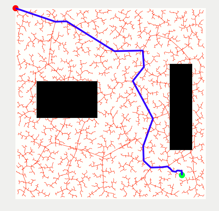
最后运行的效果是这样的:
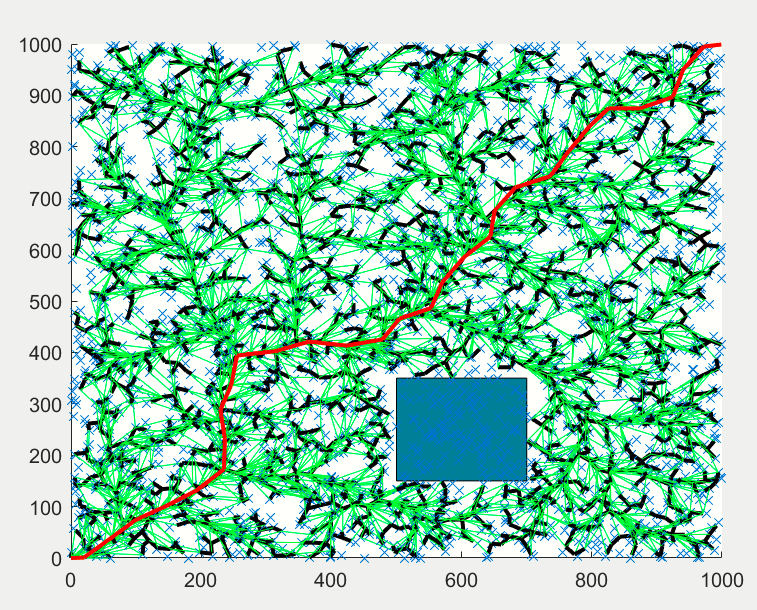
 Matlab社区中,我们也找到了参考的代码,RRT* 2D/3D
% RRT* algorithm in 2D with collision avoidance.
%
% Author: Sai Vemprala
%
% nodes:    Contains list of all explored nodes. Each node contains its
%           coordinates, cost to reach and its parent.
%
% Brief description of algorithm:
% 1. Pick a random node q_rand.
% 2. Find the closest node q_near from explored nodes to branch out from, towards
%    q_rand.
% 3. Steer from q_near towards q_rand: interpolate if node is too far away, reach
%    q_new. Check that obstacle is not hit.
% 4. Update cost of reaching q_new from q_near, treat it as Cmin. For now,
%    q_near acts as the parent node of q_new.
% 5. From the list of 'visited' nodes, check for nearest neighbors with a
%    given radius, insert in a list q_nearest.
% 6. In all members of q_nearest, check if q_new can be reached from a
%    different parent node with cost lower than Cmin, and without colliding
%    with the obstacle. Select the node that results in the least cost and
%    update the parent of q_new.
% 7. Add q_new to node list.
% 8. Continue until maximum number of nodes is reached or goal is hit.

clearvars
close all

x_max = 1000;
y_max = 1000;
obstacle = [500,150,200,200];
EPS = 20;
numNodes = 3000;

q_start.coord = [0 0];
q_start.cost = 0;
q_start.parent = 0;
q_goal.coord = [999 999];
q_goal.cost = 0;

nodes(1) = q_start;
figure(1)
axis([0 x_max 0 y_max])
rectangle('Position',obstacle,'FaceColor',[0 .5 .5])
hold on

for i = 1:1:numNodes
    q_rand = [floor(rand(1)*x_max) floor(rand(1)*y_max)];
    plot(q_rand(1), q_rand(2), 'x', 'Color',  [0 0.4470 0.7410])

    % Break if goal node is already reached
    for j = 1:1:length(nodes)
        if nodes(j).coord == q_goal.coord
            break
        end
    end

    % Pick the closest node from existing list to branch out from
    ndist = [];
    for j = 1:1:length(nodes)
        n = nodes(j);
        tmp = dist(n.coord, q_rand);
        ndist = [ndist tmp];
    end
    [val, idx] = min(ndist);
    q_near = nodes(idx);

    q_new.coord = steer(q_rand, q_near.coord, val, EPS);
    if noCollision(q_rand, q_near.coord, obstacle)
        line([q_near.coord(1), q_new.coord(1)], [q_near.coord(2), q_new.coord(2)], 'Color', 'k', 'LineWidth', 2);
        drawnow
        hold on
        q_new.cost = dist(q_new.coord, q_near.coord) + q_near.cost;

        % Within a radius of r, find all existing nodes
        q_nearest = [];
        r = 60;
        neighbor_count = 1;
        for j = 1:1:length(nodes)
            if noCollision(nodes(j).coord, q_new.coord, obstacle) && dist(nodes(j).coord, q_new.coord) <= r
                q_nearest(neighbor_count).coord = nodes(j).coord;
                q_nearest(neighbor_count).cost = nodes(j).cost;
                neighbor_count = neighbor_count+1;
            end
        end

        % Initialize cost to currently known value
        q_min = q_near;
        C_min = q_new.cost;

        % Iterate through all nearest neighbors to find alternate lower
        % cost paths

        for k = 1:1:length(q_nearest)
            if noCollision(q_nearest(k).coord, q_new.coord, obstacle) && q_nearest(k).cost + dist(q_nearest(k).coord, q_new.coord) < C_min
                q_min = q_nearest(k);
                C_min = q_nearest(k).cost + dist(q_nearest(k).coord, q_new.coord);
                line([q_min.coord(1), q_new.coord(1)], [q_min.coord(2), q_new.coord(2)], 'Color', 'g');
                hold on
            end
        end

        % Update parent to least cost-from node
        for j = 1:1:length(nodes)
            if nodes(j).coord == q_min.coord
                q_new.parent = j;
            end
        end

        % Append to nodes
        nodes = [nodes q_new];
    end
end

D = [];
for j = 1:1:length(nodes)
    tmpdist = dist(nodes(j).coord, q_goal.coord);
    D = [D tmpdist];
end

% Search backwards from goal to start to find the optimal least cost path
[val, idx] = min(D);
q_final = nodes(idx);
q_goal.parent = idx;
q_end = q_goal;
nodes = [nodes q_goal];
while q_end.parent ~= 0
    start = q_end.parent;
    line([q_end.coord(1), nodes(start).coord(1)], [q_end.coord(2), nodes(start).coord(2)], 'Color', 'r', 'LineWidth', 2);
    hold on
    q_end = nodes(start);
end
其中调用函数:
function val = ccw(A,B,C)
    val = (C(2)-A(2)) * (B(1)-A(1)) > (B(2)-A(2)) * (C(1)-A(1));
end

function d = dist(q1,q2)
d = sqrt((q1(1)-q2(1))^2 + (q1(2)-q2(2))^2);
end

function nc = noCollision(n2, n1, o)
    A = [n1(1) n1(2)];
    B = [n2(1) n2(2)];
    obs = [o(1) o(2) o(1)+o(3) o(2)+o(4)];

    C1 = [obs(1),obs(2)];
    D1 = [obs(1),obs(4)];
    C2 = [obs(1),obs(2)];
    D2 = [obs(3),obs(2)];
    C3 = [obs(3),obs(4)];
    D3 = [obs(3),obs(2)];
    C4 = [obs(3),obs(4)];
    D4 = [obs(1),obs(4)];

    % Check if path from n1 to n2 intersects any of the four edges of the
    % obstacle

    ints1 = ccw(A,C1,D1) ~= ccw(B,C1,D1) && ccw(A,B,C1) ~= ccw(A,B,D1);
    ints2 = ccw(A,C2,D2) ~= ccw(B,C2,D2) && ccw(A,B,C2) ~= ccw(A,B,D2);
    ints3 = ccw(A,C3,D3) ~= ccw(B,C3,D3) && ccw(A,B,C3) ~= ccw(A,B,D3);
    ints4 = ccw(A,C4,D4) ~= ccw(B,C4,D4) && ccw(A,B,C4) ~= ccw(A,B,D4);
    if ints1==0 && ints2==0 && ints3==0 && ints4==0
        nc = 1;
    else
        nc = 0;
    end
end

function A = steer(qr, qn, val, eps)
   qnew = [0 0];

   % Steer towards qn with maximum step size of eps
   if val >= eps
       qnew(1) = qn(1) + ((qr(1)-qn(1))*eps)/dist(qr,qn);
       qnew(2) = qn(2) + ((qr(2)-qn(2))*eps)/dist(qr,qn);
   else
       qnew(1) = qr(1);
       qnew(2) = qr(2);
   end
   A = [qnew(1), qnew(2)];
end
运行效果是这样的:
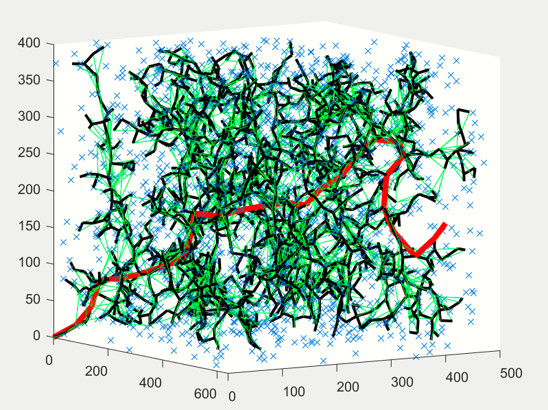
RRT* 3D
clearvars
close all
x_max = 640;
y_max = 480;
z_max = 400;

EPS = 20;
numNodes = 2000;

q_start.coord = [0 0 0];
q_start.cost = 0;
q_start.parent = 0;
q_goal.coord = [640 400 180];
q_goal.cost = 0;

nodes(1) = q_start;
figure(1)

for i = 1:1:numNodes
    q_rand = [rand(1)*x_max rand(1)*y_max rand(1)*z_max];
    plot3(q_rand(1), q_rand(2), q_rand(3), 'x', 'Color',  [0 0.4470 0.7410])

    % Break if goal node is already reached
    for j = 1:1:length(nodes)
        if nodes(j).coord == q_goal.coord
            break
        end
    end

    % Pick the closest node from existing list to branch out from
    ndist = [];
    for j = 1:1:length(nodes)
        n = nodes(j);
        tmp = dist_3d(n.coord, q_rand);
        ndist = [ndist tmp];
    end
    [val, idx] = min(ndist);
    q_near = nodes(idx);

    q_new.coord = steer3d(q_rand, q_near.coord, val, EPS);
    line([q_near.coord(1), q_new.coord(1)], [q_near.coord(2), q_new.coord(2)], [q_near.coord(3), q_new.coord(3)], 'Color', 'k', 'LineWidth', 2);
    drawnow
    hold on
    q_new.cost = dist_3d(q_new.coord, q_near.coord) + q_near.cost;

    % Within a radius of r, find all existing nodes
    q_nearest = [];
    r = 50;
    neighbor_count = 1;
    for j = 1:1:length(nodes)
        if (dist_3d(nodes(j).coord, q_new.coord)) <= r
            q_nearest(neighbor_count).coord = nodes(j).coord;
            q_nearest(neighbor_count).cost = nodes(j).cost;
            neighbor_count = neighbor_count+1;
        end
    end

    % Initialize cost to currently known value
    q_min = q_near;
    C_min = q_new.cost;

    % Iterate through all nearest neighbors to find alternate lower
    % cost paths

    for k = 1:1:length(q_nearest)
        if q_nearest(k).cost + dist_3d(q_nearest(k).coord, q_new.coord) < C_min
            q_min = q_nearest(k);
            C_min = q_nearest(k).cost + dist_3d(q_nearest(k).coord, q_new.coord);
            line([q_min.coord(1), q_new.coord(1)], [q_min.coord(2), q_new.coord(2)], [q_min.coord(3), q_new.coord(3)], 'Color', 'g');
            hold on
        end
    end

    % Update parent to least cost-from node
    for j = 1:1:length(nodes)
        if nodes(j).coord == q_min.coord
            q_new.parent = j;
        end
    end

    % Append to nodes
    nodes = [nodes q_new];
end

D = [];
for j = 1:1:length(nodes)
    tmpdist = dist_3d(nodes(j).coord, q_goal.coord);
    D = [D tmpdist];
end

% Search backwards from goal to start to find the optimal least cost path
[val, idx] = min(D);
q_final = nodes(idx);
q_goal.parent = idx;
q_end = q_goal;
nodes = [nodes q_goal];
while q_end.parent ~= 0
    start = q_end.parent;
    line([q_end.coord(1), nodes(start).coord(1)], [q_end.coord(2), nodes(start).coord(2)], [q_end.coord(3), nodes(start).coord(3)], 'Color', 'r', 'LineWidth', 4);
    hold on
    q_end = nodes(start);
end
调用的函数是:
function A = steer(qr, qn, val, eps)
   qnew = [0 0];
   if val >= eps
       qnew(1) = qn(1) + ((qr(1)-qn(1))*eps)/dist_3d(qr,qn);
       qnew(2) = qn(2) + ((qr(2)-qn(2))*eps)/dist_3d(qr,qn);
       qnew(3) = qn(3) + ((qr(3)-qn(3))*eps)/dist_3d(qr,qn);
   else
       qnew(1) = qr(1);
       qnew(2) = qr(2);
       qnew(3) = qr(3);
   end

   A = [qnew(1), qnew(2), qnew(3)];
end

function d = dist_3d(q1,q2)
    d = sqrt((q1(1)-q2(1))^2 + (q1(2)-q2(2))^2 + (q1(3)-q2(3))^2);
end
运行的结果是:
发布者:全栈程序员-用户IM,转载请注明出处:https://javaforall.cn/206664.html原文链接:https://javaforall.cn
【正版授权,激活自己账号】: Jetbrains全家桶Ide使用,1年售后保障,每天仅需1毛
【官方授权 正版激活】: 官方授权 正版激活 支持Jetbrains家族下所有IDE 使用个人JB账号...
