大家好,又见面了,我是你们的朋友全栈君。如果您正在找激活码,请点击查看最新教程,关注关注公众号 “全栈程序员社区” 获取激活教程,可能之前旧版本教程已经失效.最新Idea2022.1教程亲测有效,一键激活。
Jetbrains全家桶1年46,售后保障稳定
问题背景
近来从事毫米波雷达的定位与建图工作,想拓展下工作思路,研究autoware公司的激光点云定位与建图。期间正好发现autoware的激光点云配准算法是NDT(Normal-Distributions Transform),相比ICP算法,它能更快速高效地确定两个大型点云的刚性变换。这里分别介绍下2003年经典的2D NDT算法,以及autoware日本团队在2006年提出的3D NDT算法。
“The Normal Distributions Transform: A New Approach to Laser Scan Matching”
“A 3-D Scan Matching using Improved 3-D Normal Distributions Transform for Mobile Robotic Mapping”
二维ND
2D NDT数学描述
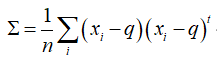
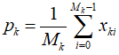
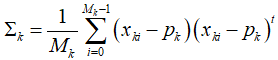
假设小车安装了只有一线的2D激光雷达,只能表达一个平面内是否有障碍物。把小车周围的区域划分成大小相同的单元格,我们可以用NDT(Normal Distribution Transform)对扫描的2D点云分布进行建模,用高斯分布表达每个单元格内2D点的聚集情况。若每个单元格包含3个以上的2D点,则计算该单元格内所有点Xi=1,…,n的坐标均值及方差。


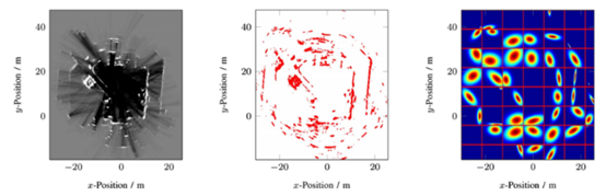
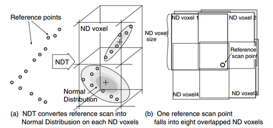
不同于于栅格图occupancy grid,NDT分布用连续可微的概率密度描述细分区域网格平面内的2D点。栅格图表达的是单元格内包含障碍物的概率,NDT分布本身表示参考帧中特定网格内2D点的位置分布情况。假设下图为参考帧,左侧时栅格图表达空与不空,中间是识别到的2D激光雷达点云,右图表达每个单元格内二维正态概率分布,每个单元格大小相同,越红的地方概率值越大。
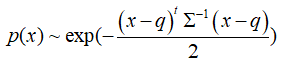
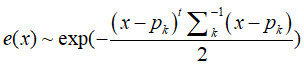
我们可以NDT分布计算当前帧新观测到的2D点坐标相对于参考帧单元格的概率(不同单元格有不同的均值和方差,均值区域表示参考帧单元格内2D点最密集的区域)。下式表示当前帧2D点x,属于参考帧中某个单元格的概率
如何划分网格并避免离散化的影响
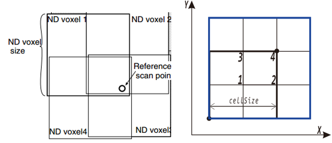
个人认为按照上图那样划分网格,破坏了2D点云结构,比如属于同一个物体的点云,被刻意分开到不同单元格计算了。这种离散化不利于地图地描述,也不利于后期点云配准。我们分别看看建图和定位时,如何划分网格,计算概率密度。
建图时,给定参考帧laser scan的2D点云,根据点云坐标上下界以及cell size确定外侧bounding box下图蓝色边框所示。对于边框内部采用4个单元格相互重叠的,两两覆盖50%,分别计算每个子网格的点云正态分布。因此这种划分包含了4种均值和方差。下右图只是示意,实际上蓝色框图内将有多个单元格,可以认为蓝色框图内大部分的2D点会同时落入四种单元格内。
定位时,计算前后两帧pose关系,给定当前帧laser scan的2D点云,根据T(待优化的参数)转换后的坐标查找落入哪个单元格内,同样当前帧每个2d点将对应四种分布。累计所有2d点对应的四种概率密度之和,通过选择合理的T,使得概率密度之和最大。
如何计算两片点云相对位姿
假设用T表达2D空间内,两个时刻机器人的位姿变换关系。下面公式表达了当前帧的2D点云在上一帧坐标系的坐标
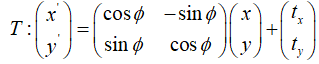
表示位移,表示旋转角度。Scan alignment目的就是通过前后两帧的laser scan复原位移和角度。假设给定两帧激光点云的测量,具体步骤如下:
(1)用第一帧laser scan,按照上述过程计算初始NDT分布
(2)初始化位姿变换参数T,全零或者用odometry初始化
(3)根据位姿变换参数T,将第二帧的laser scan点云转换到第一帧坐标系下
(4)为第二帧的每个2D点分配网格,计算点云对应的四种概率分布
(5)累计点云的概率分布,计算总体得分
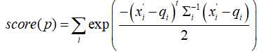
p是第二帧点云,x’是第二帧点云p经T投影在第一帧的坐标,q和sigma是x’所属第一帧的网格概率分布。
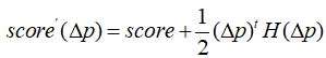
(6)用牛顿法优化参数T (任意非线性优化算法均可),使得score得分最高 [对于牛顿法,迭代步长的要点是求score函数的一阶和二阶偏导数,此处不扩展]
(7)回到步骤(3),重复上述步骤,优化算法收敛
2D NDT在SLAM中的应用
以下内容是我基于2003年那篇论文的理解,给出大致思路。
建图:
Slam地图由图结构表达,每个顶点表示当前关键帧机器人绝对位姿,顶点之间的边表示前后两帧关键帧之间2D点云经过NDT配准推算出来的relative pose(可以看作是odometry,如果有IMU或轮速传感器,就不用NDT推算前后航迹了)。地图元素就是2D 点云的正态分布(均值看作2D点云的位置,方差可看作2D点云覆盖范围),并且这些分布根据每个顶点的全局坐标,也转换到全局坐标下了。
每新增一个顶点,或者叫新增关键帧,理论上所有其他顶点都要参与全局优化。关于全局目标函数,每个顶点的全局位姿可以得到两个顶点之间相对位姿,而两个顶点对应的laser scan根据NDT匹配也能推算出相对位姿。由于全局位姿未知,我们希望通过估算两种相对位姿的差(这样能反推全局位姿),使得整体score得分最小,所以优化的目标函数是关于位姿之差的二次函数(关于score函数在NDT配准的相对位姿处二阶泰勒展开,一次项在左侧,)
另外随着关键帧增加,全局优化的顶点越来越多,无法实时计算。因此每次新增顶点,只优化三条连接边以内的子图。
定位:
假设k-n时刻的测量是关键帧,给定k-n与k时刻的里程计估计,将k时刻测量到的2D点云根据 投影到k-n时刻。通过计算k-n时刻与k时刻的NDT score,通过优化得到的位姿作为k时刻位姿。如果k时刻的测量距离k-n时刻的关键帧较远,则把最近一次NDT匹配成功的测量作为新的关键帧。
下面时matlab 工具箱内关于2D NDT Matching的代码
preNDT函数将激光数据点划分到指定大小的网格中:
function [xgridcoords, ygridcoords] = preNDT(laserScan, cellSize)
%preNDT Calculate cell coordinates based on laser scan
%   [XGRIDCOORDS, YGRIDCOORDS] = preNDT(LASERSCAN, CELLSIZE) calculated the x
%   (XGRIDCOORDS) and y (YGRIDCOORDS) coordinates of the cell center points that are
%   used to discretize the given laser scan.
%
%   Inputs:
%      LASERSCAN - N-by-2 array of 2D Cartesian points
%      CELLSIZE - Defines the side length of each cell used to build NDT.
%         Each cell is square
%
%   Outputs:
%      XGRIDCOORDS - 4-by-K, the discretized x coordinates using cells with size
%         equal to CELLSIZE.
%      YGRIDCOORDS: 4-by-K, the discretized y coordinates using cells with size
%         equal to CELLSIZE.

xmin = min(laserScan(:,1));
ymin = min(laserScan(:,2));
xmax = max(laserScan(:,1));
ymax = max(laserScan(:,2));

halfCellSize = cellSize/2;

lowerBoundX = floor(xmin/cellSize)*cellSize-cellSize;
upperBoundX = ceil(xmax/cellSize)*cellSize+cellSize;
lowerBoundY = floor(ymin/cellSize)*cellSize-cellSize;
upperBoundY = ceil(ymax/cellSize)*cellSize+cellSize;

% To minimize the effects of discretization,use four overlapping
% grids. That is, one grid with side length cellSize of a single cell is placed
% first, then a second one, shifted by cellSize/2 horizontally, a third
% one, shifted by cellSize/2 vertically and a fourth one, shifted by
% cellSize/2 horizontally and vertically.

xgridcoords = [  lowerBoundX:cellSize:upperBoundX;...                       % Grid of cells in position 1
            lowerBoundX+halfCellSize:cellSize:upperBoundX+halfCellSize;...  % Grid of cells in position 2 (X Right, Y Same)
            lowerBoundX:cellSize:upperBoundX; ...                           % Grid of cells in position 3 (X Same, Y Up)
            lowerBoundX+halfCellSize:cellSize:upperBoundX+halfCellSize];    % Grid of cells in position 4 (X Right, Y Up)

ygridcoords = [  lowerBoundY:cellSize:upperBoundY;...                     	% Grid of cells in position 1
            lowerBoundY:cellSize:upperBoundY;...                            % Grid of cells in position 2 (X Right, Y Same)
            lowerBoundY+halfCellSize:cellSize:upperBoundY+halfCellSize;...  % Grid of cells in position 3 (X Same, Y Up)
            lowerBoundY+halfCellSize:cellSize:upperBoundY+halfCellSize];    % Grid of cells in position 4 (X Right, Y Up)

endbuildNDT函数根据划分好的网格,来计算每一个小格子中的二维正态分布参数(均值、协方差矩阵以及协方差矩阵的逆):
function [xgridcoords, ygridcoords, meanq, covar, covarInv] = buildNDT(laserScan, cellSize)
%buildNDT Build Normal Distributions Transform from laser scan
%   [XGRIDCOORDS, YGRIDCOORDS, MEANQ, COVAR, COVARINV] = buildNDT(LASERSCAN, CELLSIZE)
%   discretizes the laser scan points into cells and approximates each cell
%   with a Normal distribution.
%
%   Inputs:
%      LASERSCAN - N-by-2 array of 2D Cartesian points
%      CELLSIZE - Defines the side length of each cell used to build NDT.
%         Each cell is a square area used to discretize the space.
%
%   Outputs:
%      XGRIDCOORDS - 4-by-K, the discretized x coordinates of the grid of cells,
%         with each cell having a side length equal to CELLSIZE.
%         Note that K increases when CELLSIZE decreases.
%         The second row shifts the first row by CELLSIZE/2 to
%         the right. The third row shifts the first row by CELLSIZE/2 to the
%         top. The fourth row shifts the first row by CELLSIZE/2 to the right and
%         top. The same row semantics apply to YGRIDCOORDS, MEANQ, COVAR, and COVARINV.
%      YGRIDCOORDS: 4-by-K, the discretized y coordinates of the grid of cells,
%         with each cell having a side length equal to CELLSIZE.
%      MEANQ: 4-by-K-by-K-by-2, the mean of the points in cells described by
%         XGRIDCOORDS and YGRIDCOORDS.
%      COVAR: 4-by-K-by-K-by-2-by-2, the covariance of the points in cells
%      COVARINV: 4-by-K-by-K-by-2-by-2, the inverse of the covariance of
%         the points in cells.
%
%   [XGRIDCOORDS, YGRIDCOORDS, MEANQ, COVAR, COVARINV] describe the NDT statistics.

%   Copyright 2016 The MathWorks, Inc.


% When the scan contains ONLY NaN values (no valid range readings),
% the input laserScan is empty. Explicitly
% initialize empty variables to support code generation.
if isempty(laserScan)
    xgridcoords      = zeros(4,0);
    ygridcoords      = zeros(4,0);
    meanq       = zeros(4,0,0,2);
    covar       = zeros(4,0,0,2,2);
    covarInv    = zeros(4,0,0,2,2);
    return;
end

% Discretize the laser scan into cells
[xgridcoords, ygridcoords] = preNDT(laserScan, cellSize);

xNumCells = size(xgridcoords,2);
yNumCells = size(ygridcoords,2);

% Preallocate outputs
meanq = zeros(4,xNumCells,yNumCells,2);
covar = zeros(4,xNumCells,yNumCells,2,2);
covarInv = zeros(4,xNumCells,yNumCells,2,2);

% For each cell, compute the normal distribution that can approximately
% describe the distribution of the points within the cell.
for cellShiftMode = 1:4
    % Find the points in the cell
    % First find all points in the xgridcoords and ygridcoords separately and then combine the result.
	% indx的值表示laserScan的x坐标分别在xgridcoords划分的哪个范围中(例如1就表示落在第1个区间;若不在范围中,则返回0)
    [~, indx] = histc(laserScan(:,1), xgridcoords(cellShiftMode, :));
    [~, indy] = histc(laserScan(:,2), ygridcoords(cellShiftMode, :));
    for i = 1:xNumCells
        xflags = (indx == i); % xflags is a logical vector
        for j = 1:yNumCells
            yflags = (indy == j);
            xyflags = logical(xflags .* yflags);
            xymemberInCell = laserScan(xyflags,:);  % laser points in the cell

            % If there are more than 3 points in the cell, compute the
            % statistics. Otherwise, all statistics remain zero.
            % See reference [1], section III.
            if size(xymemberInCell, 1) > 3

                % Compute mean and covariance
                xymean = mean(xymemberInCell);
                xyCov = cov(xymemberInCell, 1);

                % Prevent covariance matrix from going singular (and not be
                % invertible). See reference [1], section III.
                [U,S,V] = svd(xyCov);
                if S(2,2) < 0.001 * S(1,1)
                    S(2,2) = 0.001 * S(1,1);
                    xyCov = U*S*V';
                end

                [~, posDef] = chol(xyCov);
                if posDef ~= 0
                    % If the covariance matrix is not positive definite,
                    % disregard the contributions of this cell.
                    continue;
                end

                % Store statistics
                meanq(cellShiftMode,i,j,:) = xymean;
                covar(cellShiftMode,i,j,:,:) = xyCov;
                covarInv(cellShiftMode,i,j,:,:) = inv(xyCov);
            end
        end
    end
end
end
objectiveNDT函数根据变换参数计算目标函数值及其梯度和Hessian矩阵,objectiveNDT的输出参数将作为目标函数信息传入优化函数中:
function [score, gradient, hessian] = objectiveNDT(laserScan, laserTrans, xgridcoords, ygridcoords, meanq, covar, covarInv)
%objectiveNDT Calculate objective function for NDT-based scan matching
%   [SCORE, GRADIENT, HESSIAN] = objectiveNDT(LASERSCAN, LASERTRANS, XGRIDCOORDS,
%   YGRIDCOORDS, MEANQ, COVAR, COVARINV) calculates the NDT objective function by
%   matching the LASERSCAN transformed by LASERTRANS to the NDT described
%   by XGRIDCOORDS, YGRIDCOORDS, MEANQ, COVAR, and COVARINV.
%   The NDT score is returned in SCORE, along with the optionally
%   calculated score GRADIENT, and score HESSIAN.

%   Copyright 2016 The MathWorks, Inc.

% Create rotation matrix
theta = laserTrans(3);
sintheta = sin(theta);
costheta = cos(theta);

rotm = [costheta -sintheta;
        sintheta costheta];

% Create 2D homogeneous transform
trvec = [laserTrans(1); laserTrans(2)];
tform = [rotm, trvec
0 1];

% Create homogeneous points for laser scan
hom = [laserScan, ones(size(laserScan,1),1)];

% Apply homogeneous transform
trPts = hom * tform';  % Eqn (2)

% Convert back to Cartesian points
laserTransformed = trPts(:,1:2);

hessian = zeros(3,3);
gradient = zeros(3,1);
score = 0;

% Compute the score, gradient and Hessian according to the NDT paper
for i = 1:size(laserTransformed,1) % 对每一个转换点进行处理
    xprime = laserTransformed(i,1);
    yprime = laserTransformed(i,2);

    x = laserScan(i,1);
    y = laserScan(i,2);

    % Eqn (11)
    jacobianT = [1 0 -x*sintheta - y*costheta;
1  x*costheta - y*sintheta];

    % Eqn (13)
    qp3p3 = [-x*costheta + y*sintheta;
             -x*sintheta - y*costheta];

    for cellShiftMode = 1:4
        [~,m] = histc(xprime, xgridcoords(cellShiftMode, :)); % 转换点落在(m,n)格子中
        [~,n] = histc(yprime, ygridcoords(cellShiftMode, :));

        if m == 0 || n == 0
            continue
        end
        meanmn = reshape(meanq(cellShiftMode,m,n,:),2,1);
        covarmn = reshape(covar(cellShiftMode,m,n,:,:),2,2);
        covarmninv = reshape(covarInv(cellShiftMode,m,n,:,:),2,2);

        if ~any([any(meanmn), any(covarmn)])
            % Ignore cells that contained less than 3 points
            continue
        end

        % Eqn (3)
        q = [xprime;yprime] - meanmn;
        % As per the paper, this term should represent the probability of
        % the match of the point with the specific cell
        gaussianValue = exp(-q'*covarmninv*q/2);
        score = score - gaussianValue;

        for j = 1:3
            % Eqn (10)
            gradient(j) = gradient(j) + q'*covarmninv*jacobianT(:,j)*gaussianValue;
            % Eqn (12)
            qpj = jacobianT(:,j);
            for k = j:3           % Hessian矩阵为对称矩阵,只需要计算对角线上的部分
                qpk = jacobianT(:,k);
                if j == 3 && k == 3
                    hessian(j,k) = hessian(j,k) + gaussianValue*(-(q'*covarmninv*qpj)*(q'*covarmninv*qpk) +(q'*covarmninv*qp3p3) + (qpk'*covarmninv*qpj));
                else
                    hessian(j,k) = hessian(j,k) + gaussianValue*(-(q'*covarmninv*qpj)*(q'*covarmninv*qpk) + (qpk'*covarmninv*qpj));
                end
            end
        end
    end
end

% 补全Hessian矩阵
for j = 1:3
    for k = 1:j-1
        hessian(j,k) = hessian(k,j);
    end
end

score = double(score);
gradient = double(gradient);
hessian = double(hessian);
end
三维NDT
三维NDT分布数学描述
接下来看看NDT如何处理三维激光数据,假设有参考帧3D点集
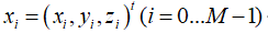
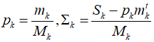
它们将被分配到称作ND voxel的三维网格中,对于第k个voxel,里面有 个3D点。对于该网格的NDT分布的均值和方差:
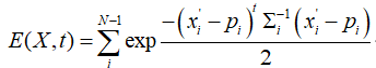
那么该网格的概率密度函数为:
如下图所示,reference点集会被三维网格包围构造多维正态分布。为了克服离散化问题,不同于2D点集,这里每个3D点会被8个三维网格包围。
3D NDT分布更新
随着地图扩张,每次三维网格内新增了参考点,均值和协方差(关于x,y,z)都会重复计算且计算量会逐渐增加。为了减少计算量,对于第k个voxel,其均值p和协方差sigma采用如下方式增量更新,计算复杂度与网格中3D点的个数无关。

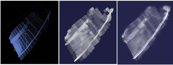
下图是3D点云对应网格的NDT可视化
如何进行3D点云NDT配准
给定两个3D点集,如何通过NDT分布计算二者的相对位姿呢?先看看三维空间的坐标变换,点集X通过(R,t)变换,R是旋转矩阵,t是平移向量

给定参考帧点云以及当前帧点云,配准问题就变成了(R,t)参数搜索问题。根据参考帧点云构造NDT分布,通过寻找合适的坐标变换参数使得当前帧点云对应的NDT概率密度之和最大。
这里同样使用牛顿优化法求解参数R和t
NDT三维网格的设计
如果三维网格voxel大小不当,那么NDT配准时会出问题。如下图所示,
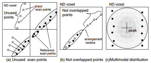
图a中黑点为参考帧,白点为当前帧,如果voxel网格尺寸太小,当前帧左上角点云没有对应的参考帧点云,对NDT配准位置修正没有贡献,反而增加了牛顿法收敛时间。另外,如果网格内点云数量过小,无法形成正态分布。
图b中,如果voxel网格尺寸较大,白色点和黑色点本不属于同一物体,虽然收敛速度很快,但是最终匹配结果是错误的。
图c中,如果voxel网格尺寸过大,网格中有两种参考点的分布,单核正态分布(单峰)不足以描述它们,所以当前帧同这种分布配准时,往往也是失败的。
如何改进
总之,网格越小,计算量越大,消耗内存大,但是匹配更精确。网格越大,计算量越小,匹配越不精确。
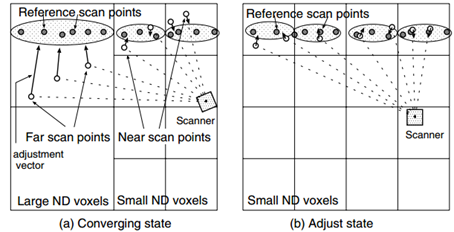
NDT TKU作者在不同计算阶段定义不同网格大小。在初始匹配时,或者叫收敛阶段,对于机器人较近激光测量采用较小的网格,而距离机器人较远的,采用较大的网格。在初始匹配完成后,进行修正阶段时,对于远处的网格将同近处测量一样采用较小的网格。因为机器人朝向角的细微差异,会导致远处测量的巨大不确定性。因此,在初始搜索匹配时,对于远处的激光点云,采用较大的网格,对于近处的点云采用较小的网格。并且最终匹配计算,将近采用较小的网格。
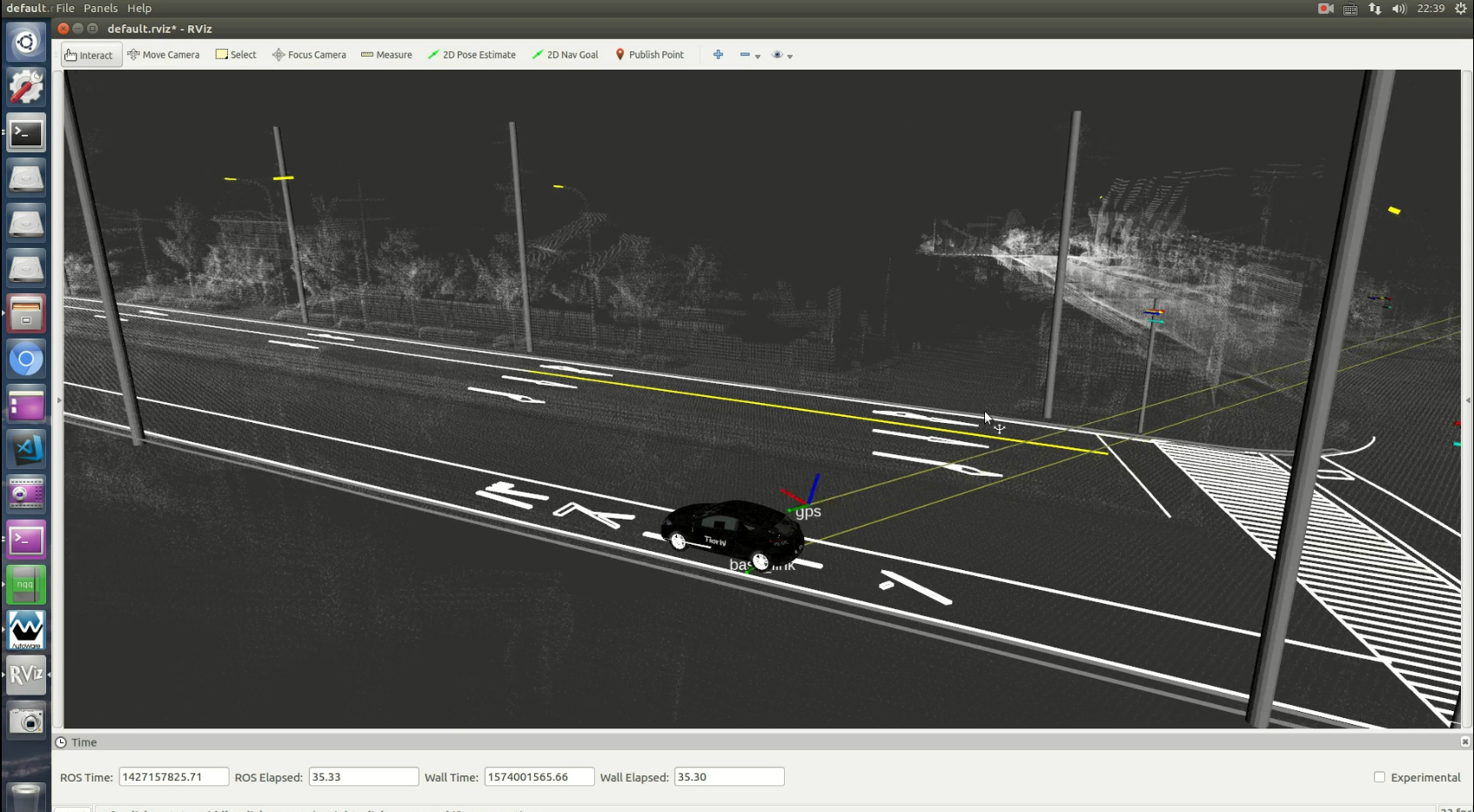
下图为autoware NDT定位截图
发布者:全栈程序员-用户IM,转载请注明出处:https://javaforall.cn/203470.html原文链接:https://javaforall.cn
【正版授权,激活自己账号】: Jetbrains全家桶Ide使用,1年售后保障,每天仅需1毛
【官方授权 正版激活】: 官方授权 正版激活 支持Jetbrains家族下所有IDE 使用个人JB账号...
