大家好，又见面了，我是你们的朋友全栈君。如果您正在找激活码,请点击查看最新教程,关注关注公众号 “全栈程序员社区” 获取激活教程,可能之前旧版本教程已经失效.最新Idea2022.1教程亲测有效,一键激活。

Jetbrains全系列IDE使用 1年只要46元 售后保障 童叟无欺

老师常说，在人工智能未发展起来之前，SVM技术是一统江湖的，SVM常常听到，但究竟是什么呢？最近研究了一下基于SVM技术的手写数字识别。你没有看错，又是手写数字识别，就是喜欢这个手写数字识别，没办法(￢∀￢)σ

一、背景

1.手写数字识别技术的含义

2.手写数字识别技术的理论价值

3.数字识别技术的难点

二、SVM技术

1.SVM方法简介

 2.线性可划分问题

3.近似线性可分问题的线性划分

4.非线性划分

5.SVM方法

6.SVM的性能

三、实验

1.数据集介绍

2.实验步骤

3.实验代码

4.实验结果

四、附录

1.参考

2.需要安装的包

一、背景

1.手写数字识别技术的含义

手写数字识别(Handwritten Digit Recognition)是光学字符识别技术的一个分支，是模式识别学科的一个传统研究领域。主要研究如何利用电子计算机自动辨认手写在纸张上的阿拉伯数字。手写数字识别分为脱机手写数字识别和联机手写数字识别。本文主要讨论脱机手写数字的识别。 随着信息化的发展，手写数字识别的应用日益广泛，研究高识别率、零误识率和低拒识率的高速识别算法具有重要意义。

2.手写数字识别技术的理论价值

由于手写数字识别本身的特点，对它的研究有重要的理论价值：

 ⑴阿拉伯数字是唯一被世界各国通用的符号，对手写体数字识别的研究基本上与文化背景无关，各地的研究工作者基于同一平台开展工作，有利于研究的比较和探讨。

 ⑵手写数字识别应用广泛，如邮政编码自动识别，税表系统和银行支票自动处理等。这些工作以前需要大量的手工录入，投入的人力物力较多，劳动强度较大。手写数字识别的研究适应了无纸化办公的需要，能大大提高工作效率。

⑶由于数字类别只有 10 个，较其他字符识别率较高，可用于验证新的理论和做深入的分析研究。许多机器学习和模式识别领域的新理论和算法都是先用手写数字识别进行检验，验证理论的有效性，然后才应用到更复杂的领域当中。这方面的典型例子就是人工神经网络和支持向量机(Support Vector Machine)。

 ⑷手写数字的识别方法很容易推广到其它一些相关问题，如对英文之类拼音文字的识别。事实上，很多学者就是把数字和英文字母的识别放在一起研究的。

3.数字识别技术的难点

数字的类别只有 10 种，笔划简单，其识别问题似乎不是很困难。但事实上，一些测试结果表明，数字的正确识别率并不如印刷体汉字识别率高，甚至也不如联机手写体汉字识别率高，而只仅仅优于脱机手写体汉字识别。这其中的主要原因是：

⑴数字笔划简单，其笔划差别相对较小，字形相差不大，使得准确区分某些数字相当困难；

⑵数字虽然只有 10 种，且笔划简单，但同一数字写法千差万别，全世界各个国家各个地区的人都在用，其书写上带有明显的区域特性，很难做出可以兼顾世界各种写法的、识别率极高的通用性数字识别系统。

虽然目前国内外对脱机手写数字识别的研究已经取得了很大的成就，但是仍然存在两大难点：

一是识别精度需要达到更高的水平。手写数字识别没有上下文，数据中的每一个数据都至关重要。而数字识别经常涉及金融、财会领域，其严格性更是不言而喻。因此，国内外众多的学者都在为提高手写数字的识别率，降低误识率而努力。

二是识别的速度要达到很高的水平。数字识别的输入通常是很大量的数据，而高精度与高速度是相互矛盾的，因此对识别算法提出了更高的要求。

二、SVM技术

1.SVM方法简介

统计学习理论是建立在一套较坚实的理论基础之上的,为解决有限样本学习问题提供了一个统一的框架。它能将很多现有方法纳入其中,有望解决许多原来难以解决的问题比如神经网络结构选择问题、局部极小点问题等同时,在该理论基础上发展了一种新的通用学习方法——支持向量机（SupportVectorMachine，简称SVM）,已初步表现出很多优于己有方法的性能。一些学者认为正在成为继神经网络研究之后新的研究热点,并将推动机器学习理论和技术有重大的发展。

SVM方法是建立在统计学习理论的维理论和结构风险最小化原理基础上的,根据有限的样本信息在模型的复杂性即对特定训练样本的学习精度和学习能力即无误识别任意样本的能力之间寻求最佳折衷,以期获得最好的推广能力。

 2.线性可划分问题

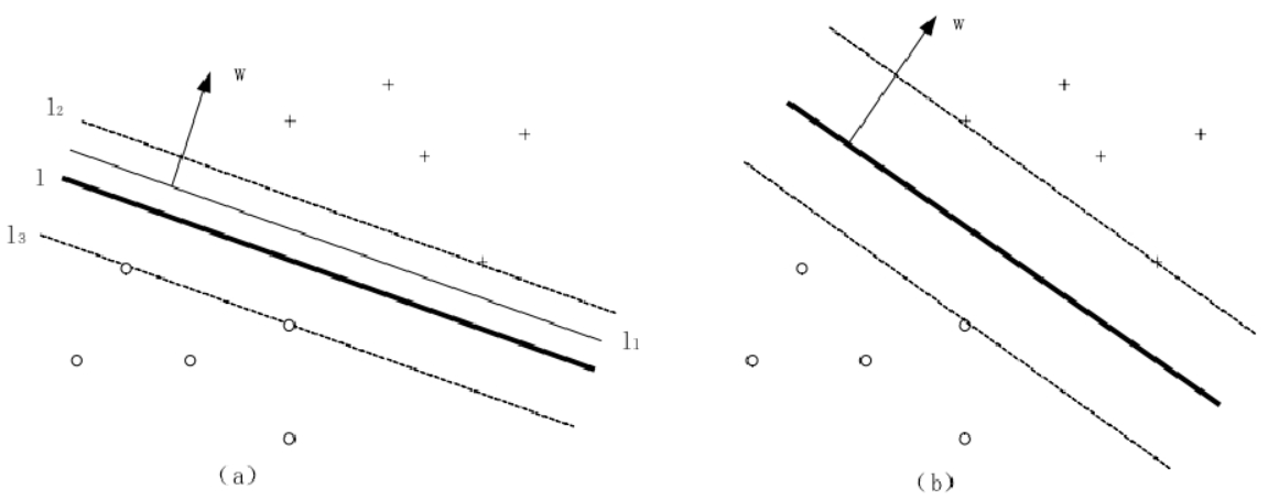
                                                                                                   图1最大间隔法

3.近似线性可分问题的线性划分

4.非线性划分

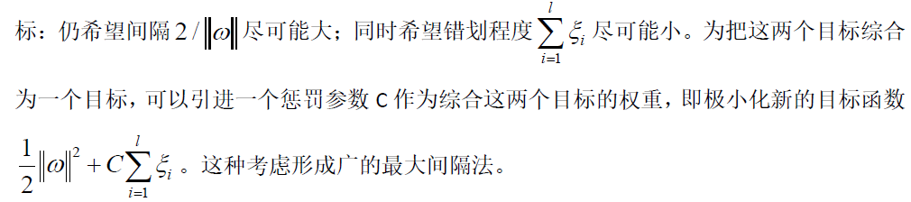
讲到这里，做个思路整理：首先，面对线性可划分问题，我们可以很容易利用最大间隔法，找到最优分类面，将数据分成两类。面对有些线性不可分问题，我们找不到这样一个最优分类面，但是在我们允许很小程度上的错分后，我们可以找到一个最优分类面。这时我们寻找的依据处理要求间隔最大，还要错分的程度最小，这个要求统称为惩罚参数。最后，面对其他线性不可分问题，我们实在找不到一个最优分类面的情况下，我们需要先做一些非线性变换，将非线性问题转化为线性问题，然后再进行处理。

5.SVM方法

 

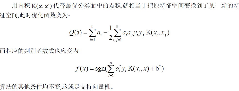
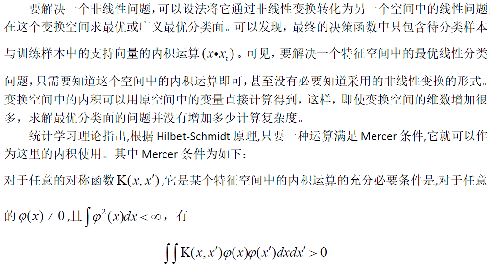
SVM的基本思想可以概括为首先通过非线性变换将输入空间变换到一个高维空间,然后在这个新空间中求取最优线性分类面,而这种非线性变换是通过定义适当的内积函数实现的。

SVM求得的分类函数形式上类似于一个神经网络,其输出的若干中间层节点的线性组合,而每一个中间层节点对应于输入样本与一个支持向量机的内积,因此也被称为支持向量网络。

由于最终判决函数中实际只包含与支持向量的内积和求和,因此识别时的计算复杂度取决于支持向量的个数。

另一个问题的关键是,由于变换空间的维数可能很高,在这个空间中的线性判别函数的VC维因此也可能很大,将导致分类器的效果不理想。而只要在高维空间中能够构造一个具有较小的VC维,从而得到较好的推广能力。

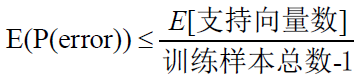
进一步,关于最优分类面和广义最优分类面的推广能力,有下面的结论：

如果一组训练样本能够被一个最优分类面或广义最优分类面分开,对于测试样本分类错误率的期望的上界是训练样本中平均的支持向量占总训练样本数的比例,即

SVM推广性也是与变换空间的维数无关的,只要能够适当地选择一种内积定义,构造一个支持向量数相对较少的最优或广义最优分类器,则就可以得到较好的推广性。

在这里,统计学习理论使用了与传统方法完全不同的思路,即不是像传统方法那样首先试图将原输入空间降维即特征选择和特征变换,而是设法将输入空间升维,以求在高维空间中问题变得线性可分或接近线性可分因为升维后只是改变了内积运算,并没有使算法复杂性随着维数的增加而增加,而且在高维空间中的推广能力并不受维数影响,因此这种方法才是可行的。

6.SVM的性能

使用SVM方法，需要做特征空间的内积运算，而核函数就是內积。SVM核函数的选择对于其性能的表现有至关重要的作用，尤其是针对那些线性不可分的数据，因此核函数的选择在SVM算法中就显得至关重要。常用如下几种常用的核函数来代替自己构造核函数：

（1）线性核函数 

线性核主要用于线性可分的情况，我们可以看到特征空间到输入空间的维度是一样的，其参数少速度快，对于线性可分数据，其分类效果很理想。

（2）多项式核函数 

多项式核函数可以实现将低维的输入空间映射到高纬的特征空间，但是多项式核函数的参数多，当多项式的阶数比较高的时候，核矩阵的元素值将趋于无穷大或者无穷小，计算复杂度会大到无法计算。

（3）高斯（RBF）核函数

高斯径向基函数是一种局部性强的核函数，其可以将一个样本映射到一个更高维的空间内，该核函数是应用最广的一个，无论大样本还是小样本都有比较好的性能，而且其相对于多项式核函数参数要少，因此大多数情况下在不知道用什么核函数的时候，优先使用高斯核函数。

（4）sigmoid核函数

采用sigmoid核函数，支持向量机实现的就是一种多层神经网络。

除了核函数的选取，SVM的策略对SVM的性能也十分重要。手写数字字体识别，显然是个多类别分类问题。对于多分类问题，解决的基本思路是“拆分法”，即将多个二分类问题拆分为若干个十分类任务进行求解。具体来讲，先对问题进行拆分，然后为拆出的每个十分类任务训练一个分类器，在测试时，对这些二分类器的结果进行集成以获得最终的多分类结果。拆分的策略主要有以下几种：

（1）OvO（one-vs-one）

这种解决方法的思路是：对于有N个类别的分类任任务，将这N个类别两两配对，从而产生N(N-1)/2个二分类任务。在测试阶段，新样本同时提交给所有分类器，这样可以得到N(N-1)/2个分类结果，最终的结果可以通过投票产生：即把预测的最多的类别作为最终的分类结果。

（2）OvR（one-vs-rest）

这种解决方法的思路是：每次将一个类的样例作为正例，所有其他类的样例作为负例来训练N个分类器。在测试时，若仅有一个分类器预测为正类，则对应的类别标记为最终分类结果。

三、实验

1.数据集介绍

本文采用MNIST-image手写数字集进行训练和测试。MNIST数据集是机器学习领域中非常经典的一个数据集，由60000个训练样本和10000个测试样本组成，每个样本都是一张20 * 20像素的灰度手写数字图片。数字已经过尺寸标准化，并以固定尺寸的图像为中心。数据如图2：

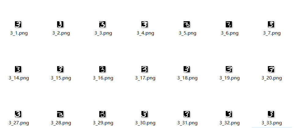
                                                                                图2 MNIST-image数据集

2.实验步骤

（1）对数据格式转换
（2）使用核函数和训练策略对训练集进行训练
（3）使用训练后得到的模型对测试集进行测试
（4）选择最佳核函数和训练策略为模型
（5）用此模型进行可视化识别

3.实验代码

（1）训练svm模型并保存

from PIL import Image
import os
import sys
import numpy as np
import time
from sklearn import svm
from sklearn.externals import joblib

# 获取指定路径下的所有 .png 文件
def get_file_list(path):
    # file_list = []
    # for filename in os.listdir(path):
    #     ele_path = os.path.join(path, filename)
    #     for imgname in os.listdir(ele_path):
    #         subele_path = os.path.join(ele_path, imgname)
    #         if (subele_path.endswith(".png")):
    #             file_list.append(subele_path)
    # return file_list
    return [os.path.join(path, f) for f in os.listdir(path) if f.endswith(".png")]



# 解析出 .png 图件文件的名称
def get_img_name_str(imgPath):
    return imgPath.split(os.path.sep)[-1]


# 将 20px * 20px 的图像数据转换成 1*400 的 numpy 向量
# 参数：imgFile--图像名  如：0_1.png
# 返回：1*400 的 numpy 向量
def img2vector(imgFile):
    # print("in img2vector func--para:{}".format(imgFile))
    img = Image.open(imgFile).convert('L')
    img_arr = np.array(img, 'i')  # 20px * 20px 灰度图像
    img_normalization = np.round(img_arr / 255)  # 对灰度值进行归一化
    img_arr2 = np.reshape(img_normalization, (1, -1))  # 1 * 400 矩阵
    return img_arr2


# 读取一个类别的所有数据并转换成矩阵
# 参数：
#    basePath: 图像数据所在的基本路径
#       Mnist-image/train/
#       Mnist-image/test/
#    cla：类别名称
#       0,1,2,...,9
# 返回：某一类别的所有数据----[样本数量*(图像宽x图像高)] 矩阵
def read_and_convert(imgFileList):
    dataLabel = []  # 存放类标签
    dataNum = len(imgFileList)
    dataMat = np.zeros((dataNum, 400))  # dataNum * 400 的矩阵
    for i in range(dataNum):
        imgNameStr = imgFileList[i]
        imgName = get_img_name_str(imgNameStr)  # 得到 数字_实例编号.png
        # print("imgName: {}".format(imgName))
        classTag = imgName.split(".")[0].split("_")[0]  # 得到 类标签(数字)
        # print("classTag: {}".format(classTag))
        dataLabel.append(classTag)
        dataMat[i, :] = img2vector(imgNameStr)
    return dataMat, dataLabel


# 读取训练数据
def read_all_data():
    cName = ['1', '2', '3', '4', '5', '6', '7', '8', '9']
    path = sys.path[1]
    train_data_path = os.path.join(path, 'data\\Mnist-image\\train\
from PIL import Image
import os
import sys
import numpy as np
import time
from sklearn import svm
from sklearn.externals import joblib
# 获取指定路径下的所有 .png 文件
def get_file_list(path):
# file_list = []
# for filename in os.listdir(path):
#     ele_path = os.path.join(path, filename)
#     for imgname in os.listdir(ele_path):
#         subele_path = os.path.join(ele_path, imgname)
#         if (subele_path.endswith(".png")):
#             file_list.append(subele_path)
# return file_list
return [os.path.join(path, f) for f in os.listdir(path) if f.endswith(".png")]
# 解析出 .png 图件文件的名称
def get_img_name_str(imgPath):
return imgPath.split(os.path.sep)[-1]
# 将 20px * 20px 的图像数据转换成 1*400 的 numpy 向量
# 参数：imgFile--图像名  如：0_1.png
# 返回：1*400 的 numpy 向量
def img2vector(imgFile):
# print("in img2vector func--para:{}".format(imgFile))
img = Image.open(imgFile).convert('L')
img_arr = np.array(img, 'i')  # 20px * 20px 灰度图像
img_normalization = np.round(img_arr / 255)  # 对灰度值进行归一化
img_arr2 = np.reshape(img_normalization, (1, -1))  # 1 * 400 矩阵
return img_arr2
# 读取一个类别的所有数据并转换成矩阵
# 参数：
#    basePath: 图像数据所在的基本路径
#       Mnist-image/train/
#       Mnist-image/test/
#    cla：类别名称
#       0,1,2,...,9
# 返回：某一类别的所有数据----[样本数量*(图像宽x图像高)] 矩阵
def read_and_convert(imgFileList):
dataLabel = []  # 存放类标签
dataNum = len(imgFileList)
dataMat = np.zeros((dataNum, 400))  # dataNum * 400 的矩阵
for i in range(dataNum):
imgNameStr = imgFileList[i]
imgName = get_img_name_str(imgNameStr)  # 得到 数字_实例编号.png
# print("imgName: {}".format(imgName))
classTag = imgName.split(".")[0].split("_")[0]  # 得到 类标签(数字)
# print("classTag: {}".format(classTag))
dataLabel.append(classTag)
dataMat[i, :] = img2vector(imgNameStr)
return dataMat, dataLabel
# 读取训练数据
def read_all_data():
cName = ['1', '2', '3', '4', '5', '6', '7', '8', '9']
path = sys.path[1]
train_data_path = os.path.join(path, 'data\\Mnist-image\\train\\0')
#print(train_data_path)
#train_data_path = "Mnist-image\\train\\0"
print('0')
flist = get_file_list(train_data_path)
dataMat, dataLabel = read_and_convert(flist)
for c in cName:
print(c)
train_data_path = os.path.join(path, 'data\\Mnist-image\\train\\') + c
flist_ = get_file_list(train_data_path)
dataMat_, dataLabel_ = read_and_convert(flist_)
dataMat = np.concatenate((dataMat, dataMat_), axis=0)
dataLabel = np.concatenate((dataLabel, dataLabel_), axis=0)
# print(dataMat.shape)
# print(len(dataLabel))
return dataMat, dataLabel
# create model
def create_svm(dataMat, dataLabel,path,decision='ovr'):
clf = svm.SVC(C=1.0,kernel='rbf',decision_function_shape=decision)
rf =clf.fit(dataMat, dataLabel)
joblib.dump(rf, path)
return clf
'''
SVC参数
svm.SVC(C=1.0,kernel='rbf',degree=3,gamma='auto',coef0=0.0,shrinking=True,probability=False,
tol=0.001,cache_size=200,class_weight=None,verbose=False,max_iter=-1,decision_function_shape='ovr',random_state=None)
C：C-SVC的惩罚参数C?默认值是1.0
C越大，相当于惩罚松弛变量，希望松弛变量接近0，即对误分类的惩罚增大，趋向于对训练集全分对的情况，这样对训练集测试时
准确率很高，但泛化能力弱。C值小，对误分类的惩罚减小，允许容错，将他们当成噪声点，泛化能力较强。
kernel ：核函数，默认是rbf，可以是‘linear’, ‘poly’, ‘rbf’, ‘sigmoid’, ‘precomputed’ 
0 – 线性：u'v
 　　 1 – 多项式：(gamma*u'*v + coef0)^degree
  　　2 – RBF函数：exp(-gamma|u-v|^2)
  　　3 –sigmoid：tanh(gamma*u'*v + coef0)
degree ：多项式poly函数的维度，默认是3，选择其他核函数时会被忽略。（没用）
gamma ： ‘rbf’,‘poly’ 和‘sigmoid’的核函数参数。默认是’auto’，则会选择1/n_features
coef0 ：核函数的常数项。对于‘poly’和 ‘sigmoid’有用。（没用）
probability ：是否采用概率估计？.默认为False
shrinking ：是否采用shrinking heuristic方法，默认为true
tol ：停止训练的误差值大小，默认为1e-3
cache_size ：核函数cache缓存大小，默认为200
class_weight ：类别的权重，字典形式传递。设置第几类的参数C为weight*C(C-SVC中的C)
verbose ：允许冗余输出？
max_iter ：最大迭代次数。-1为无限制。
decision_function_shape ：‘ovo’, ‘ovr’ or None, default=None3（选用ovr，一对多）
random_state ：数据洗牌时的种子值，int值
主要调节的参数有：C、kernel、degree、gamma、coef0
'''
if __name__ == '__main__':
# clf = svm.SVC(decision_function_shape='ovr')
st = time.clock()
dataMat, dataLabel = read_all_data()
path = sys.path[1]
model_path=os.path.join(path,'model\\svm.model')
create_svm(dataMat, dataLabel,model_path, decision='ovr')
et = time.clock()
print("Training spent {:.4f}s.".format((et - st)))
')
    #print(train_data_path)
    #train_data_path = "Mnist-image\\train\
from PIL import Image
import os
import sys
import numpy as np
import time
from sklearn import svm
from sklearn.externals import joblib
# 获取指定路径下的所有 .png 文件
def get_file_list(path):
# file_list = []
# for filename in os.listdir(path):
#     ele_path = os.path.join(path, filename)
#     for imgname in os.listdir(ele_path):
#         subele_path = os.path.join(ele_path, imgname)
#         if (subele_path.endswith(".png")):
#             file_list.append(subele_path)
# return file_list
return [os.path.join(path, f) for f in os.listdir(path) if f.endswith(".png")]
# 解析出 .png 图件文件的名称
def get_img_name_str(imgPath):
return imgPath.split(os.path.sep)[-1]
# 将 20px * 20px 的图像数据转换成 1*400 的 numpy 向量
# 参数：imgFile--图像名  如：0_1.png
# 返回：1*400 的 numpy 向量
def img2vector(imgFile):
# print("in img2vector func--para:{}".format(imgFile))
img = Image.open(imgFile).convert('L')
img_arr = np.array(img, 'i')  # 20px * 20px 灰度图像
img_normalization = np.round(img_arr / 255)  # 对灰度值进行归一化
img_arr2 = np.reshape(img_normalization, (1, -1))  # 1 * 400 矩阵
return img_arr2
# 读取一个类别的所有数据并转换成矩阵
# 参数：
#    basePath: 图像数据所在的基本路径
#       Mnist-image/train/
#       Mnist-image/test/
#    cla：类别名称
#       0,1,2,...,9
# 返回：某一类别的所有数据----[样本数量*(图像宽x图像高)] 矩阵
def read_and_convert(imgFileList):
dataLabel = []  # 存放类标签
dataNum = len(imgFileList)
dataMat = np.zeros((dataNum, 400))  # dataNum * 400 的矩阵
for i in range(dataNum):
imgNameStr = imgFileList[i]
imgName = get_img_name_str(imgNameStr)  # 得到 数字_实例编号.png
# print("imgName: {}".format(imgName))
classTag = imgName.split(".")[0].split("_")[0]  # 得到 类标签(数字)
# print("classTag: {}".format(classTag))
dataLabel.append(classTag)
dataMat[i, :] = img2vector(imgNameStr)
return dataMat, dataLabel
# 读取训练数据
def read_all_data():
cName = ['1', '2', '3', '4', '5', '6', '7', '8', '9']
path = sys.path[1]
train_data_path = os.path.join(path, 'data\\Mnist-image\\train\\0')
#print(train_data_path)
#train_data_path = "Mnist-image\\train\\0"
print('0')
flist = get_file_list(train_data_path)
dataMat, dataLabel = read_and_convert(flist)
for c in cName:
print(c)
train_data_path = os.path.join(path, 'data\\Mnist-image\\train\\') + c
flist_ = get_file_list(train_data_path)
dataMat_, dataLabel_ = read_and_convert(flist_)
dataMat = np.concatenate((dataMat, dataMat_), axis=0)
dataLabel = np.concatenate((dataLabel, dataLabel_), axis=0)
# print(dataMat.shape)
# print(len(dataLabel))
return dataMat, dataLabel
# create model
def create_svm(dataMat, dataLabel,path,decision='ovr'):
clf = svm.SVC(C=1.0,kernel='rbf',decision_function_shape=decision)
rf =clf.fit(dataMat, dataLabel)
joblib.dump(rf, path)
return clf
'''
SVC参数
svm.SVC(C=1.0,kernel='rbf',degree=3,gamma='auto',coef0=0.0,shrinking=True,probability=False,
tol=0.001,cache_size=200,class_weight=None,verbose=False,max_iter=-1,decision_function_shape='ovr',random_state=None)
C：C-SVC的惩罚参数C?默认值是1.0
C越大，相当于惩罚松弛变量，希望松弛变量接近0，即对误分类的惩罚增大，趋向于对训练集全分对的情况，这样对训练集测试时
准确率很高，但泛化能力弱。C值小，对误分类的惩罚减小，允许容错，将他们当成噪声点，泛化能力较强。
kernel ：核函数，默认是rbf，可以是‘linear’, ‘poly’, ‘rbf’, ‘sigmoid’, ‘precomputed’ 
0 – 线性：u'v
 　　 1 – 多项式：(gamma*u'*v + coef0)^degree
  　　2 – RBF函数：exp(-gamma|u-v|^2)
  　　3 –sigmoid：tanh(gamma*u'*v + coef0)
degree ：多项式poly函数的维度，默认是3，选择其他核函数时会被忽略。（没用）
gamma ： ‘rbf’,‘poly’ 和‘sigmoid’的核函数参数。默认是’auto’，则会选择1/n_features
coef0 ：核函数的常数项。对于‘poly’和 ‘sigmoid’有用。（没用）
probability ：是否采用概率估计？.默认为False
shrinking ：是否采用shrinking heuristic方法，默认为true
tol ：停止训练的误差值大小，默认为1e-3
cache_size ：核函数cache缓存大小，默认为200
class_weight ：类别的权重，字典形式传递。设置第几类的参数C为weight*C(C-SVC中的C)
verbose ：允许冗余输出？
max_iter ：最大迭代次数。-1为无限制。
decision_function_shape ：‘ovo’, ‘ovr’ or None, default=None3（选用ovr，一对多）
random_state ：数据洗牌时的种子值，int值
主要调节的参数有：C、kernel、degree、gamma、coef0
'''
if __name__ == '__main__':
# clf = svm.SVC(decision_function_shape='ovr')
st = time.clock()
dataMat, dataLabel = read_all_data()
path = sys.path[1]
model_path=os.path.join(path,'model\\svm.model')
create_svm(dataMat, dataLabel,model_path, decision='ovr')
et = time.clock()
print("Training spent {:.4f}s.".format((et - st)))
"
    print('0')
    flist = get_file_list(train_data_path)
    dataMat, dataLabel = read_and_convert(flist)
    for c in cName:
        print(c)
        train_data_path = os.path.join(path, 'data\\Mnist-image\\train\\') + c
        flist_ = get_file_list(train_data_path)
        dataMat_, dataLabel_ = read_and_convert(flist_)
        dataMat = np.concatenate((dataMat, dataMat_), axis=0)
        dataLabel = np.concatenate((dataLabel, dataLabel_), axis=0)
    # print(dataMat.shape)
    # print(len(dataLabel))
    return dataMat, dataLabel


# create model
def create_svm(dataMat, dataLabel,path,decision='ovr'):
    clf = svm.SVC(C=1.0,kernel='rbf',decision_function_shape=decision)
    rf =clf.fit(dataMat, dataLabel)
    joblib.dump(rf, path)
    return clf
'''
SVC参数
svm.SVC(C=1.0,kernel='rbf',degree=3,gamma='auto',coef0=0.0,shrinking=True,probability=False,
tol=0.001,cache_size=200,class_weight=None,verbose=False,max_iter=-1,decision_function_shape='ovr',random_state=None)

C：C-SVC的惩罚参数C?默认值是1.0
C越大，相当于惩罚松弛变量，希望松弛变量接近0，即对误分类的惩罚增大，趋向于对训练集全分对的情况，这样对训练集测试时
准确率很高，但泛化能力弱。C值小，对误分类的惩罚减小，允许容错，将他们当成噪声点，泛化能力较强。
kernel ：核函数，默认是rbf，可以是‘linear’, ‘poly’, ‘rbf’, ‘sigmoid’, ‘precomputed’ 
       0 – 线性：u'v
 　　 1 – 多项式：(gamma*u'*v + coef0)^degree
  　　2 – RBF函数：exp(-gamma|u-v|^2)
  　　3 –sigmoid：tanh(gamma*u'*v + coef0)
degree ：多项式poly函数的维度，默认是3，选择其他核函数时会被忽略。（没用）
gamma ： ‘rbf’,‘poly’ 和‘sigmoid’的核函数参数。默认是’auto’，则会选择1/n_features
coef0 ：核函数的常数项。对于‘poly’和 ‘sigmoid’有用。（没用）
probability ：是否采用概率估计？.默认为False
shrinking ：是否采用shrinking heuristic方法，默认为true
tol ：停止训练的误差值大小，默认为1e-3
cache_size ：核函数cache缓存大小，默认为200
class_weight ：类别的权重，字典形式传递。设置第几类的参数C为weight*C(C-SVC中的C)
verbose ：允许冗余输出？
max_iter ：最大迭代次数。-1为无限制。
decision_function_shape ：‘ovo’, ‘ovr’ or None, default=None3（选用ovr，一对多）
random_state ：数据洗牌时的种子值，int值
主要调节的参数有：C、kernel、degree、gamma、coef0

'''

if __name__ == '__main__':
    # clf = svm.SVC(decision_function_shape='ovr')
    st = time.clock()
    dataMat, dataLabel = read_all_data()
    path = sys.path[1]
    model_path=os.path.join(path,'model\\svm.model')
    create_svm(dataMat, dataLabel,model_path, decision='ovr')
    et = time.clock()
    print("Training spent {:.4f}s.".format((et - st)))

（2）测试模型效果

import sys
import time
import svm
import os
from sklearn.externals import joblib
import numpy as np
import matplotlib.pyplot as plt


def svmtest(model_path):
    path = sys.path[1]
    tbasePath = os.path.join(path, "data\\Mnist-image\\test\\")
    tcName = ['0', '1', '2', '3', '4', '5', '6', '7', '8', '9']
    tst = time.clock()
    allErrCount = 0
    allErrorRate = 0.0
    allScore = 0.0
    ErrCount=np.zeros(10,int)
    TrueCount=np.zeros(10,int)
    #加载模型
    clf = joblib.load(model_path)
    for tcn in tcName:
        testPath = tbasePath + tcn
        # print("class " + tcn + " path is: {}.".format(testPath))
        tflist = svm.get_file_list(testPath)
        # tflist
        tdataMat, tdataLabel = svm.read_and_convert(tflist)
        print("test dataMat shape: {0}, test dataLabel len: {1} ".format(tdataMat.shape, len(tdataLabel)))
        # print("test dataLabel: {}".format(len(tdataLabel)))
        pre_st = time.clock()
        preResult = clf.predict(tdataMat)
        pre_et = time.clock()
        print("Recognition  " + tcn + " spent {:.4f}s.".format((pre_et - pre_st)))
        # print("predict result: {}".format(len(preResult)))
        errCount = len([x for x in preResult if x != tcn])
        ErrCount[int(tcn)]=errCount
        TrueCount[int(tcn)]= len(tdataLabel)-errCount
        print("errorCount: {}.".format(errCount))
        allErrCount += errCount
        score_st = time.clock()
        score = clf.score(tdataMat, tdataLabel)
        score_et = time.clock()
        print("computing score spent {:.6f}s.".format(score_et - score_st))
        allScore += score
        print("score: {:.6f}.".format(score))
        print("error rate is {:.6f}.".format((1 - score)))

    tet = time.clock()
    print("Testing All class total spent {:.6f}s.".format(tet - tst))
    print("All error Count is: {}.".format(allErrCount))
    avgAccuracy = allScore / 10.0
    print("Average accuracy is: {:.6f}.".format(avgAccuracy))
    print("Average error rate is: {:.6f}.".format(1 - avgAccuracy))
    print("number"," TrueCount"," ErrCount")
    for tcn in tcName:
        tcn=int(tcn)
        print(tcn,"     ",TrueCount[tcn],"      ",ErrCount[tcn])
    plt.figure(figsize=(12, 6))
    x=list(range(10))
    plt.plot(x,TrueCount, color='blue', label="TrueCount")  # 将正确的数量设置为蓝色
    plt.plot(x,ErrCount, color='red', label="ErrCount")  # 将错误的数量为红色
    plt.legend(loc='best')  # 显示图例的位置，这里为右下方
    plt.title('Projects')
    plt.xlabel('number')  # x轴标签
    plt.ylabel('count')  # y轴标签
    plt.xticks(np.arange(10), ['0', '1', '2', '3', '4', '5', '6', '7', '8', '9'])
    plt.show()


if __name__ == '__main__':
    path = sys.path[1]
    model_path=os.path.join(path,'model\\svm.model')
    svmtest(model_path)

（3）可视化

# -*- coding: utf-8 -*-

# Form implementation generated from reading ui file 'test2.ui'
#
# Created by: PyQt5 UI code generator 5.11.3
#
# WARNING! All changes made in this file will be lost!

import sys
from PyQt5.QtWidgets import QApplication, QMainWindow,QFileDialog
from PyQt5 import QtCore, QtGui, QtWidgets
from PyQt5.QtGui import *
from PyQt5.QtWidgets import *
from PyQt5.QtCore import *
import os
from sklearn.externals import joblib
import svm
class Ui_Dialog(object):
    def setupUi(self, Dialog):
        Dialog.setObjectName("Dialog")
        Dialog.resize(645, 475)
        self.pushButton = QtWidgets.QPushButton(Dialog)
        self.pushButton.setGeometry(QtCore.QRect(230, 340, 141, 41))
        self.pushButton.setAutoDefault(False)
        self.pushButton.setObjectName("pushButton")
        self.label = QtWidgets.QLabel(Dialog)
        self.label.setGeometry(QtCore.QRect(220, 50, 191, 221))
        self.label.setWordWrap(False)
        self.label.setObjectName("label")
        self.textEdit = QtWidgets.QTextEdit(Dialog)
        self.textEdit.setGeometry(QtCore.QRect(220, 280, 191, 41))
        self.textEdit.setObjectName("textEdit")

        self.retranslateUi(Dialog)
        QtCore.QMetaObject.connectSlotsByName(Dialog)

    def retranslateUi(self, Dialog):
        _translate = QtCore.QCoreApplication.translate
        Dialog.setWindowTitle(_translate("Dialog", "手写体识别"))
        self.pushButton.setText(_translate("Dialog", "打开图片"))
        self.label.setText(_translate("Dialog", "显示图片"))

class MyWindow(QMainWindow, Ui_Dialog):
    def __init__(self, parent=None):
        super(MyWindow, self).__init__(parent)
        self.setupUi(self)
        self.pushButton.clicked.connect(self.openImage)

    def openImage(self):
        imgName, imgType = QFileDialog.getOpenFileName(self, "打开图片", "../data/Mnist-image/test")
        png = QtGui.QPixmap(imgName).scaled(self.label.width(), self.label.height())
        self.label.setPixmap(png)
        self.textEdit.setText(imgName)

        path = sys.path[1]
        model_path = os.path.join(path, 'model\\svm.model')
        clf = joblib.load(model_path)
        dataMat=svm.img2vector(imgName)
        preResult = clf.predict(dataMat)
        self.textEdit.setReadOnly(True)
        self.textEdit.setStyleSheet("color:red")
        self.textEdit.setAlignment(QtCore.Qt.AlignHCenter|QtCore.Qt.AlignVCenter)
        self.textEdit.setFontPointSize(9)
        self.textEdit.setText("预测的结果是：")
        self.textEdit.append(preResult[0])

if __name__ == '__main__':
    app = QApplication(sys.argv)
    myWin = MyWindow()
    myWin.show()
    sys.exit(app.exec_())

4.实验结果

将MNIST-image数据集运用SVM进行识别，我们选择以线性核函数、RBF核函数、Sigmoid核函数为核函数，以OVO和OVR为策略，两两搭配，共有六种组合，以这六种组合分别训练和测试数据集，并记录其训练时间、测试时间、准确率和平均准确率，得到如下两表：

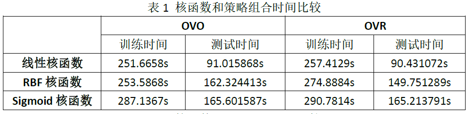
从表1可以看出，三种核函数的训练时间和测试时间排序是：线性核函数<RBF核函数<Sigmoid核函数;OVO策略的训练时间小于OVR的训练时间，而OVR的测试时间小于OVO的测试时间。

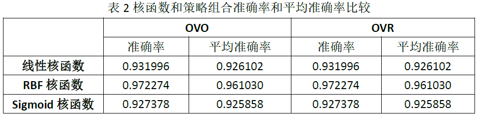
从表2可以看出，三种核函数的准确率排序是：RBF核函数>线性核函数>Sigmoid核函数。三种核函数的平均准确率排序是：RBF核函数>线性核函数>Sigmoid核函数.OVO和OVR的准确率和错误率一样。

造成核函数和策略组合性能不同的原因如下：

（1）线性核函数、RBF核函数和Sigmoid核函数公式的复杂度不同，导致训练时间和测试时间出现差异。

（2）理论上，OVR只需要训练N个分类器，而OVO需要训练N(N-1)/2个分类器，因此OVO的存储开销和测试时间开销通常比OVR更大。而在训练时，OVR的每个分类器均使用全部训练样例，而OVO的每个分类器仅用到两个类的样例。因此，在类别很多的时候，OVO的训练时间开销通常比OVR更小。

（3）手写数字识别中，各种数字写法复杂，这明显是线性不可分的情景，所以线性核函数的准确率较低。

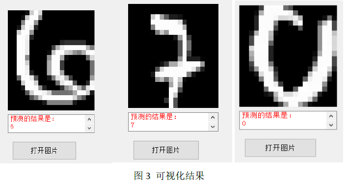
可视化结果如图3所示：

最优模型的各个数字情况如图4、表3所示：

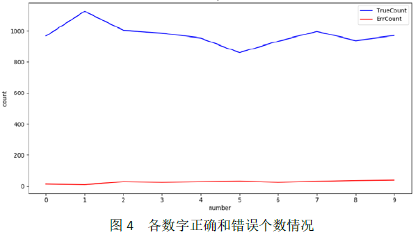
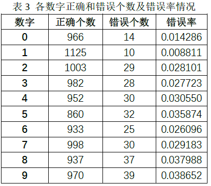
从表3中我们可以看出，各数字整体的错误率都不高，但数字9、8、5、4的错误率是最高的四个，错误率达3%以上，原因是以为这些数字写法相对灵活多变，书写不规范，造成识别率低，这也是今后要加强的地方。

四、附录

1.参考

https://blog.csdn.net/ni_guang2010/article/details/53069579

https://blog.csdn.net/w5688414/article/details/79343542

https://blog.csdn.net/rozol/article/details/87705426

基于SVM技术的手写数字识别的研究_吴琳琳

SVM在手写数字识别中的应用研究_李雅琴

2.需要安装的包

博主的电脑是win10系统，python版本是3.6

（1）pip install numpy

（2）pip install Pillow

（3）python -m pip install –upgrade pip

（4）pip install scipy

（5）pip3 install sklearn

（6）pip install PyQt5

（7）pip3.6 install PyQt5-tools

（8）pip install matplotlib

安装教程

（1）python3.6+pyQt5+QtDesigner简易安装教程 – Rocket_J的博客 – CSDN博客

             https://blog.csdn.net/Rocket_J/article/details/80897367

（2）python3+PyQt5+Qt designer+pycharm安装及配置+将ui文件转py文件 – lyzwjaa的博客 – CSDN博客 

             https://blog.csdn.net/lyzwjaa/article/details/79429901