代码解读器_网页代码解读

大家好，又见面了，我是你们的朋友全栈君。如果您正在找激活码,请点击查看最新教程,关注关注公众号 “全栈程序员社区” 获取激活教程,可能之前旧版本教程已经失效.最新Idea2022.1教程亲测有效,一键激活。

Jetbrains全系列IDE稳定放心使用

0 写在前面

在对STN的原论文进行了翻译、理解后，我打算去github上运行下源码，以加深对ST的理解。毕竟，talk is cheap，show me the code！

此外，虽然论文作者发布是tf的源码，但由于我对tensorflow不如pytorch熟稔，因此这里我只看了pytorch官网复现的STN代码。发现写得非常详细，很适合小白入门，因此我放弃了自己解读的机会，打算就搬运一下原教程哈哈。

1 具体教程

注：以下内容均为复制/翻译，不过我在代码上加了点中文注释

Spatial transformer networks（简称STN）允许神经网络学习如何对输入图像执行空间变换，以增强模型的几何不变性。 例如，它可以裁剪感兴趣的区域，缩放并校正图像的方向。 这是一个有用的机制，因为CNN不会对旋转和缩放以及更一般的仿射变换保持invariance。

1.1 导入库

# License: BSD
# Author: Ghassen Hamrouni


from __future__ import print_function # 即使在python2.X，使用print就得像python3.X那样加括号使用
import torch
import torch.nn as nn
import torch.nn.functional as F
import torch.optim as optim
import torchvision
from torchvision import datasets, transforms
import matplotlib.pyplot as plt
import numpy as np

plt.ion()   # interactive mode

1.2 载入数据

在这个教程中我们使用MNIST手写数据集。

device = torch.device("cuda" if torch.cuda.is_available() else "cpu")

# Training dataset
train_loader = torch.utils.data.DataLoader(
    datasets.MNIST(root='.', train=True, download=True,
                   transform=transforms.Compose([
                       transforms.ToTensor(),
                       transforms.Normalize((0.1307,), (0.3081,))
                   ])), batch_size=64, shuffle=True, num_workers=4)
# Test dataset
test_loader = torch.utils.data.DataLoader(
    datasets.MNIST(root='.', train=False, transform=transforms.Compose([
        transforms.ToTensor(),
        transforms.Normalize((0.1307,), (0.3081,))
    ])), batch_size=64, shuffle=True, num_workers=4)

个人觉得难懂的地方：
1.Pytorch MNIST数据集标准化为什么是transforms.Normalize((0.1307,), (0.3081,))

1.3 建立STN模型

class Net(nn.Module):
def __init__(self):
super(Net, self).__init__()
self.conv1 = nn.Conv2d(1, 10, kernel_size=5)  # in_channel, out_channel, kennel_size
self.conv2 = nn.Conv2d(10, 20, kernel_size=5)
self.conv2_drop = nn.Dropout2d()
self.fc1 = nn.Linear(320, 50)
self.fc2 = nn.Linear(50, 10)
# Spatial transformer localization-network
# 其实这里的localization-network也只是一个普通的CNN+全连接层
# nn.Conv2d前几个参数为in_channel, out_channel, kennel_size, stride=1, padding=0
# nn.MaxPool2d前几个参数为kernel_size, stride=None, padding=0, dilation=1, return_indices=False, ceil_mode=False
self.localization = nn.Sequential(
nn.Conv2d(in_channels=1, out_channels=8, kernel_size=7),
nn.MaxPool2d(2, stride=2),
nn.ReLU(True),
nn.Conv2d(8, 10, kernel_size=5),
nn.MaxPool2d(2, stride=2),
nn.ReLU(True)
)
# Regressor for the 3 * 2 affine matrix
self.fc_loc = nn.Sequential(
nn.Linear(10 * 3 * 3, 32),  # in_features, out_features, bias = True
nn.ReLU(True),
nn.Linear(32, 3 * 2)
)
# Initialize the weights/bias with identity transformation
self.fc_loc[2].weight.data.zero_()
self.fc_loc[2].bias.data.copy_(torch.tensor([1, 0, 0, 0, 1, 0], dtype=torch.float))
# Spatial transformer network forward function
def stn(self, x):
xs = self.localization(x)  # 先进入localization层
xs = xs.view(-1, 10 * 3 * 3)  # 展开为向量
theta = self.fc_loc(xs)  # 进入全连接层，得到theta向量
theta = theta.view(-1, 2, 3)  # 对theta向量进行resize操作，输出2*3的仿射变换矩阵,通道数为C
# affine_grid函数的输入中，theta的格式为(N,2,3)，size参数的格式为(N,C,W',H')
# affine_grid函数中得到的输出grid的大小为(N,H,W,2)，这里的2是因为一个点的坐标需要x和y两个数来描述
grid = F.affine_grid(theta=theta, size=x.size())  # 这里size参数为输出图像的大小，和输入一样，因此采取x.size
# grid_sample函数的输入中，x代表ST的输入图，格式为(N,C,W,H),W'可以不等于W,H‘可以不等于H;grid是上一步得到的
x = F.grid_sample(x, grid)
return x
def forward(self, x):
# transform the input
x = self.stn(x)
# Perform the usual forward pass
x = F.relu(F.max_pool2d(self.conv1(x), 2))
x = F.relu(F.max_pool2d(self.conv2_drop(self.conv2(x)), 2))
x = x.view(-1, 320)
x = F.relu(self.fc1(x))
x = F.dropout(x, training=self.training)
x = self.fc2(x)
return F.log_softmax(x, dim=1)
model = Net().to(device)

个人觉得难懂的地方：
1.localization net中卷积层的尺寸问题。经过计算，最后一个卷积池的输入是7×7，理论上没法池化呀，硬是要池化的话，输出难道为“3.5×3.5”个像素吗？实际上，由于maxpool层中ceil_mode=False，也就是会舍弃无法整除的部分，因此下面代码的第三行中，xs.view是1033，其中10代表MNIST有十个分类，3*3代表经过最后一个池化层的图片尺寸。

def stn(self, x):
xs = self.localization(x)  # 先进入localization层
xs = xs.view(-1, 10 * 3 * 3)  # 展开为向量

具体计算过程如下：

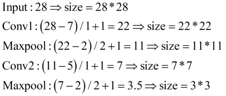
此外，输入MNIST是单通道的（C=1)，经过localization net后变为了10通道，这点代码里写得很清楚。

2.grid部分函数的输出和输出尺寸。（1）F.affine_grid。当时这一块我没太看懂，仔细阅读了下文档看懂了。F.affine_grid函数生成网格，一般输入两个参数，其中参数theta的尺寸为(N,2,3)，参数size的尺寸为(N,C,W’,H’)，N代表一次性输入的图片数量，C代表通道数目；affine_grid函数得到的输出grid的大小为(N,H,W,2)，这里的2是因为一个点的坐标需要x和y两个数来描述；官方教程给出的代码中是采取了size=x.size()，意思是这里size参数为输出图像的大小，和输入一样，实际操作中W’可以不等于W,H’可以不等于H;（2）F.grid_sample。利用上一步得到的网络在grid在原图上采样，输出(N,C,W’,H’)的图片。

grid = F.affine_grid(theta=theta, size=x.size())  # 得到网络grid
x = F.grid_sample(x, grid)  # 利用grid在原图上采样

1.4 训练部分

这里就是标准的深度学习网络。
网上看到很多人在问ST如何训练，其实不需要特别训练，把ST加入到你自己的CNN它就会自己进行反向传播调整参数的。

optimizer = optim.SGD(model.parameters(), lr=0.01)
def train(epoch):
model.train()
for batch_idx, (data, target) in enumerate(train_loader):
data, target = data.to(device), target.to(device)
optimizer.zero_grad()
output = model(data)
loss = F.nll_loss(output, target)  # 前面用的是log_softmax，因此这里用nll_loss
loss.backward()
optimizer.step()
if batch_idx % 500 == 0:
print('Train Epoch: {} [{}/{} ({:.0f}%)]\tLoss: {:.6f}'.format(
epoch, batch_idx * len(data), len(train_loader.dataset),
100. * batch_idx / len(train_loader), loss.item()))
#
# A simple test procedure to measure STN the performances on MNIST.
#
def test():
with torch.no_grad():
model.eval()
test_loss = 0
correct = 0
for data, target in test_loader:
data, target = data.to(device), target.to(device)
output = model(data)
# sum up batch loss
test_loss += F.nll_loss(output, target, reduction='sum').item()
# get the index of the max log-probability
pred = output.max(1, keepdim=True)[1]
correct += pred.eq(target.view_as(pred)).sum().item()
test_loss /= len(test_loader.dataset)
print('\nTest set: Average loss: {:.4f}, Accuracy: {}/{} ({:.0f}%)\n'
.format(test_loss, correct, len(test_loader.dataset),
100. * correct / len(test_loader.dataset)))

个人觉得难懂的地方：
1.为什么loss要用nll_loss？因为前面用了log_softmax。

1.5 可视化&运行！

def convert_image_np(inp):
"""Convert a Tensor to numpy image."""
inp = inp.numpy().transpose((1, 2, 0))
mean = np.array([0.485, 0.456, 0.406])
std = np.array([0.229, 0.224, 0.225])
inp = std * inp + mean
inp = np.clip(inp, 0, 1)
return inp
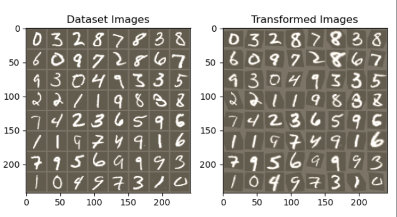
# We want to visualize the output of the spatial transformers layer
# after the training, we visualize a batch of input images and
# the corresponding transformed batch using STN.
def visualize_stn():
with torch.no_grad():
# Get a batch of training data
data = next(iter(test_loader))[0].to(device)
input_tensor = data.cpu()
transformed_input_tensor = model.stn(data).cpu()
in_grid = convert_image_np(
torchvision.utils.make_grid(input_tensor))
out_grid = convert_image_np(
torchvision.utils.make_grid(transformed_input_tensor))
# Plot the results side-by-side
f, axarr = plt.subplots(1, 2)
axarr[0].imshow(in_grid)
axarr[0].set_title('Dataset Images')
axarr[1].imshow(out_grid)
axarr[1].set_title('Transformed Images')
if __name__ == '__main__':
for epoch in range(1, 20 + 1):
train(epoch)
test()
# Visualize the STN transformation on some input batch
visualize_stn()
plt.ioff()
plt.show()

2 运行结果

只截取了部分。

————————————————————————————
Train Epoch: 19 [0/60000 (0%)] Loss: 0.097642
Train Epoch: 19 [32000/60000 (53%)] Loss: 0.092502
Test set: Average loss: 0.0388, Accuracy: 9871/10000 (99%)
————————————————————————————
Train Epoch: 20 [0/60000 (0%)] Loss: 0.042493
Train Epoch: 20 [32000/60000 (53%)] Loss: 0.025031
Test set: Average loss: 0.0396, Accuracy: 9874/10000 (99%)
————————————————————————————

3 完整代码，复制即可运行！

有问题可以咨询我，或者去原教程看哈。

# License: BSD
# Author: Ghassen Hamrouni
#%% 导入库
from __future__ import print_function  # 即使在python2.X，使用print就得像python3.X那样加括号使用
import torch
import torch.nn as nn
import torch.nn.functional as F
import torch.optim as optim
import torchvision
from torchvision import datasets, transforms
import matplotlib.pyplot as plt
import numpy as np
#%% 加载数据
device = torch.device("cuda" if torch.cuda.is_available() else "cpu")
# Training dataset
train_loader = torch.utils.data.DataLoader(
datasets.MNIST(root='.', train=True, download=True,
transform=transforms.Compose([
transforms.ToTensor(),
transforms.Normalize((0.1307,), (0.3081,))
])), batch_size=64, shuffle=True, num_workers=4)
# Test dataset
test_loader = torch.utils.data.DataLoader(
datasets.MNIST(root='.', train=False, transform=transforms.Compose([
transforms.ToTensor(),
transforms.Normalize((0.1307,), (0.3081,))
])), batch_size=64, shuffle=True, num_workers=4)
#%% 建立模型
class Net(nn.Module):
def __init__(self):
super(Net, self).__init__()
self.conv1 = nn.Conv2d(1, 10, kernel_size=5)  # in_channel, out_channel, kennel_size
self.conv2 = nn.Conv2d(10, 20, kernel_size=5)
self.conv2_drop = nn.Dropout2d()
self.fc1 = nn.Linear(320, 50)
self.fc2 = nn.Linear(50, 10)
# Spatial transformer localization-network
# 其实这里的localization-network也只是一个普通的CNN+全连接层
# nn.Conv2d前几个参数为in_channel, out_channel, kennel_size, stride=1, padding=0
# nn.MaxPool2d前几个参数为kernel_size, stride=None, padding=0, dilation=1, return_indices=False, ceil_mode=False
self.localization = nn.Sequential(
nn.Conv2d(in_channels=1, out_channels=8, kernel_size=7),
nn.MaxPool2d(2, stride=2),
nn.ReLU(True),
nn.Conv2d(8, 10, kernel_size=5),
nn.MaxPool2d(2, stride=2),
nn.ReLU(True)
)
# Regressor for the 3 * 2 affine matrix
self.fc_loc = nn.Sequential(
nn.Linear(10 * 3 * 3, 32),  # in_features, out_features, bias = True
nn.ReLU(True),
nn.Linear(32, 3 * 2)
)
# Initialize the weights/bias with identity transformation
self.fc_loc[2].weight.data.zero_()
self.fc_loc[2].bias.data.copy_(torch.tensor([1, 0, 0, 0, 1, 0], dtype=torch.float))
# Spatial transformer network forward function
def stn(self, x):
xs = self.localization(x)  # 先进入localization层
xs = xs.view(-1, 10 * 3 * 3)  # 展开为向量
theta = self.fc_loc(xs)  # 进入全连接层，得到theta向量
theta = theta.view(-1, 2, 3)  # 对theta向量进行resize操作，输出2*3的仿射变换矩阵,通道数为C
# affine_grid函数的输入中，theta的格式为(N,2,3)，size参数的格式为(N,C,W',H')
# affine_grid函数中得到的输出grid的大小为(N,H,W,2)，这里的2是因为一个点的坐标需要x和y两个数来描述
grid = F.affine_grid(theta=theta, size=x.size())  # 这里size参数为输出图像的大小，和输入一样，因此采取x.size
# grid_sample函数的输入中，x代表ST的输入图，格式为(N,C,W,H),W'可以不等于W,H‘可以不等于H;grid是上一步得到的
x = F.grid_sample(x, grid)
return x
def forward(self, x):
# transform the input
x = self.stn(x)
# Perform the usual forward pass
x = F.relu(F.max_pool2d(self.conv1(x), 2))
x = F.relu(F.max_pool2d(self.conv2_drop(self.conv2(x)), 2))
x = x.view(-1, 320)
x = F.relu(self.fc1(x))
x = F.dropout(x, training=self.training)
x = self.fc2(x)
return F.log_softmax(x, dim=1)
model = Net().to(device)
#%% 训练模型
optimizer = optim.SGD(model.parameters(), lr=0.01)
def train(epoch):
model.train()
for batch_idx, (data, target) in enumerate(train_loader):
data, target = data.to(device), target.to(device)
optimizer.zero_grad()
output = model(data)
loss = F.nll_loss(output, target)  # 前面用的是log_softmax，因此这里用nll_loss
loss.backward()
optimizer.step()
if batch_idx % 500 == 0:
print('Train Epoch: {} [{}/{} ({:.0f}%)]\tLoss: {:.6f}'.format(
epoch, batch_idx * len(data), len(train_loader.dataset),
100. * batch_idx / len(train_loader), loss.item()))
#
# A simple test procedure to measure STN the performances on MNIST.
#
def test():
with torch.no_grad():
model.eval()
test_loss = 0
correct = 0
for data, target in test_loader:
data, target = data.to(device), target.to(device)
output = model(data)
# sum up batch loss
test_loss += F.nll_loss(output, target, reduction='sum').item()
# get the index of the max log-probability
pred = output.max(1, keepdim=True)[1]
correct += pred.eq(target.view_as(pred)).sum().item()
test_loss /= len(test_loader.dataset)
print('\nTest set: Average loss: {:.4f}, Accuracy: {}/{} ({:.0f}%)\n'
.format(test_loss, correct, len(test_loader.dataset),
100. * correct / len(test_loader.dataset)))
#%% Visualizing the STN results
def convert_image_np(inp):
"""Convert a Tensor to numpy image."""
inp = inp.numpy().transpose((1, 2, 0))
mean = np.array([0.485, 0.456, 0.406])
std = np.array([0.229, 0.224, 0.225])
inp = std * inp + mean
inp = np.clip(inp, 0, 1)
return inp
# We want to visualize the output of the spatial transformers layer
# after the training, we visualize a batch of input images and
# the corresponding transformed batch using STN.
def visualize_stn():
with torch.no_grad():
# Get a batch of training data
data = next(iter(test_loader))[0].to(device)
input_tensor = data.cpu()
transformed_input_tensor = model.stn(data).cpu()
in_grid = convert_image_np(
torchvision.utils.make_grid(input_tensor))
out_grid = convert_image_np(
torchvision.utils.make_grid(transformed_input_tensor))
# Plot the results side-by-side
f, axarr = plt.subplots(1, 2)
axarr[0].imshow(in_grid)
axarr[0].set_title('Dataset Images')
axarr[1].imshow(out_grid)
axarr[1].set_title('Transformed Images')
if __name__ == '__main__':
for epoch in range(1, 20 + 1):
train(epoch)
test()
# Visualize the STN transformation on some input batch
visualize_stn()
plt.ioff()
plt.show()