大家好，又见面了，我是你们的朋友全栈君。如果您正在找激活码,请点击查看最新教程,关注关注公众号 “全栈程序员社区” 获取激活教程,可能之前旧版本教程已经失效.最新Idea2022.1教程亲测有效,一键激活。

Jetbrains全系列IDE稳定放心使用

最近在做天线多目标优化的实例，因此接触到了NSGA-Ⅱ算法，所以想分享以下我个人的学习内容与经历，仅作参考，如果内容有误，也希望各位能够指出来，大家一起进行交流指正。
内容将分为以下几个模块，内容可能较多，如果觉得不错的话，可以点赞?，收藏或者转发哦！

NSGA-Ⅱ算法简介

NSGA-Ⅱ算法由Deb等人首次提出，其思想为带有精英保留策略的快速非支配多目标优化算法，是一种基于Pareto最优解的多目标优化算法。
该算法的重要过程为：将进化群体按照支配关系分成若干层，第一层为进化群体中的非支配个体集合，第二层为在进化群体中去掉第一层个体后求得非支配个体集合，第三层，第四层依此类推。
在这里，我就不再赘述NSGA-Ⅱ的具体概念，而是将重点放在如何实现上。想要进行初步学习的可以转至：作者 晓风wangchao，标题 多目标优化算法（一）NSGA-Ⅱ（NSGA2）
支配集与非支配集的了解可以参考书籍：《多目标进化优化》或者自行百度，csdn中其他的文章。个人觉得这是基本的概念哈，可以自学。
可行解为符合约束条件的解，不可行解为不符合约束条件的解。
需要注意的是，本文讲解的是带约束条件的多目标优化，因此程序中也会掺和一些约束条件，NSGA-Ⅱ适用于解决3维及以下的多目标优化问题，即优化目标不大于3。
关于NSGA-Ⅱ带约束的matlab代码网上已经有公开的资源了，在这里用到的是MATLAB code for Constrained NSGA II – Dr.S.Baskar, S. Tamilselvi and P.R.Varshini

主程序代码：

%% Description
% 1. This is the main program of NSGA II. It requires only one input, which is test problem
%    index, 'p'. NSGA II code is tested and verified for 14 test problems.
% 2. This code defines population size in 'pop_size', number of design
%    variables in 'V', number of runs in 'no_runs', maximum number of 
%    generations in 'gen_max', current generation in 'gen_count' and number of objectives
%    in 'M'.
% 3. 'xl' and 'xu' are the lower and upper bounds of the design variables.
% 4. Final optimal Pareto soutions are in the variable 'pareto_rank1', with design
%    variables in the coumns (1:V), objectives in the columns (V+1 to V+M),
%    constraint violation in the column (V+M+1), Rank in (V+M+2), Distance in (V+M+3).
%% code starts
M = 2;%目标函数的个数
pop_size= 100;%种群数
no_runs = 10;%过程循环次数
gen_max=500;%最大迭代次数
V = 3;%变量个数
xl = [72.6,69.2,6.5,13.8,3];
xu = [75.2,73.5,9.7,16.4,6];
etac = 20;%交叉操作的分布指标
etam = 100;%编译操作的分布指标
pm = 1/V;%变异率
Q = [];%将每次循环得到的帕累托前沿保存
ref_point = [-10,-5]
for run = 1:no_runs
%初始化种群数
xl_temp=repmat(xl, pop_size,1);
xu_temp=repmat(xu, pop_size,1);
x = xl_temp+((xu_temp-xl_temp).*rand(pop_size,V));
for i =1:pop_size
[ff(i,:) err(i,:)] =feval(fname, x(i,:));           % Objective function evaulation 
end
error_norm=normalisation(err);
population_init=[x ff error_norm];
[population front]=NDSCD_cons(population_init);
%迭代开始
for gen_count=1:gen_max
% 选择
parent_selected=binary_tour_selection(population);%二项锦标赛选择
% 繁殖，生成后代
child_offspring  = genetic_operator(parent_selected(:,1:V));
for i =1:pop_size
[fff(i,:) err(i,:)] =feval(fname, x(i,:));           % Objective function evaulation 
end
error_norm=normalisation(err);
child_offspring=[child_offspring fff error_norm];
%子代与父代合并，种群数为2N
population_inter=[population(:,1:V+M+1) ; child_offspring(:,1:V+M+1)];
[population_inter_sorted front]=NDS_CD_cons(population_inter);%非支配解排序并计算聚集距离
%精英保留策略选出N个个体，组成新的一代种群
new_pop=replacement(population_inter_sorted, front);
population=new_pop;
%% 计算超立方体积（Hypervolume）指标
pop = sortrows(new_pop,V+1);
index = find(pop(:,V+M+2)==1);
non_dominated_front = pop(index,V+1:V+2);
hypervolume(gen_count+1) = Hypervolume(non_dominated_front,ref_point);
plot(non_dominated_front(:,1),non_dominated_front(:,2),'*')
set(gca,'YScale','log')
title('NSGAII: Tradeoff')
xlabel('objective function 1')
ylabel('objective function 2')
axis square
drawnow
pause(1)
end
paretoset(run).trial=new_pop(:,1:V+M+1);
Q = [Q; paretoset(run).trial]; 
end
% 绘制帕累托面
if run==1
index = find(new_pop(:,V+M+2)==1);
non_dominated_front = new_pop(index,V+1:V+2);
plot(non_dominated_front(:,1),non_dominated_front(:,2),'*')
else                                        
[pareto_filter front]=NDS_CD_cons(Q);               % Applying non domination sorting on the combined Pareto solution set
rank1_index=find(pareto_filter(:,V+M+2)==1);        % Filtering the best solutions of rank 1 Pareto
pareto_rank1=pareto_filter(rank1_index,1:V+M);
plot(pareto_rank1(:,V+1),pareto_rank1(:,V+2),'*')   % Final Pareto plot
end
xlabel('objective function 1')
ylabel('objective function 2')

本例采用该代码进行2目标约束优化，并且是求得最小值。

非支配集排序

在文献[1]中针对约束函数的情况进行了非支配偏序排序规定：
①任何可行解比任何不可行解具有更好的非支配等级；
②所有的可行解根据目标函数值计算聚集距离，聚集距离越大具有约好的等级；
③对于不可行解，具有更小的约束函数违反值的排序优先。

先贴上代码：

%% Description
% 1. This function is to perform Deb's fast elitist non-domination sorting and crowding distance assignment. 
% 2. Input is in the variable 'population' with size: [size(popuation), V+M+1]
% 3. This function returns 'chromosome_NDS_CD' with size [size(population),V+M+4]
% 4. A flag 'problem_type' is used to identify whether the population is fully feasible (problem_type=0) or fully infeasible (problem_type=1) 
%    or partly feasible (problem_type=0.5). 
%% Reference:
%Kalyanmoy Deb, Amrit Pratap, Sameer Agarwal, and T. Meyarivan, " A Fast and Elitist Multiobjective Genetic Algorithm: NSGA-II", 
%IEEE TRANSACTIONS ON EVOLUTIONARY COMPUTATION, VOL. 6, No. 2, APRIL 2002. 
%% Function part
function [chromosome_NDS_CD front] = NDSCD_cons(population)
global V M problem_type 
%% Initialising structures and variables
chromosome_NDS_CD1=[];
infpop=[];
front.fr=[];
struct.sp=[];
rank=1;
%% 将可行解与不可行解分开
if all(population(:,V+M+1)==0) %种群中所有都是可行解的情况
problem_type=0;
chromosome=population(:,1:V+M);                            
pop_size1=size(chromosome,1);%可行解个数
elseif all(population(:,V+M+1)~=0) %种群中所有都是不可行解的情况
problem_type=1;
pop_size1=0;
infchromosome=population;
else                            %种群中既有可行解也有不可行解的情况
problem_type=0.5;
feas_index=find(population(:,V+M+1)==0);
chromosome=population(feas_index,1:V+M);%可行解的约束违反值可忽略
pop_size1=size(chromosome,1);%找出种群中的可行解
infeas_index=find(population(:,V+M+1)~=0);
infchromosome=population(infeas_index,1:V+M+1);%找出种群中的不可行解
end
%% 先解决可行解
if problem_type==0 | problem_type==0.5
pop_size1 = size(chromosome,1);% 得到可行解的个数
f1 = chromosome(:,V+1);%obj1
f2 = chromosome(:,V+2);%obj2
f3 = chromosome(:,V+3);%obj3
%% 构造非支配解集并进行排序
%第一部分
for p=1:pop_size1
struct(p).sp=find(((f1(p)-f1)<0 &(f2(p)-f2)<0) | ((f2(p)-f2)==0 &(f1(p)-f1)<0) | ((f1(p)-  f1)==0 &(f2(p)-f2)<0)); 
n(p)=length(find(((f1(p)-f1)>0 &(f2(p)-f2)>0) | ((f2(p)-f2)==0 &(f1(p)-f1)>0) | ((f1(p)-f1)==0 &(f2(p)-f2)>0)));
end
front(1).fr=find(n==0);
%构造接下来的部分
while (~isempty(front(rank).fr))
front_indiv=front(rank).fr;
n(front_indiv)=inf;
chromosome(front_indiv,V+M+1)=rank;
rank=rank+1;
front(rank).fr=[];
for i = 1:length(front_indiv)
temp=struct(front_indiv(i)).sp;
n(temp)=n(temp)-1;
end
q=find(n==0);
front(rank).fr=[front(rank).fr q];
end
chromosome_sorted=sortrows(chromosome,V+M+1)';%根据rank排序
%% 计算个体之间的聚集距离
rowsindex=1;
for i = 1:length(front)-1
l_f=length(front(i).fr);
if l_f > 2
sorted_indf1=[];
sorted_indf2=[];
sortedf1=[];
sortedf2=[];
%根据f1,f2,f3的值排列
[sortedf1 sorted_indf1]=sortrows(chromosome_sorted(rowsindex:(rowsindex+l_f-1),V+1));
[sortedf2 sorted_indf2]=sortrows(chromosome_sorted(rowsindex:(rowsindex+l_f-1),V+2));
f1min=chromosome_sorted(sorted_indf1(1)+rowsindex-1,V+1);
f1max=chromosome_sorted(sorted_indf1(end)+rowsindex-1,V+1);
chromosome_sorted(sorted_indf1(1)+rowsindex-1,V+M+2)=inf;
chromosome_sorted(sorted_indf1(end)+rowsindex-1,V+M+2)=inf;
f2min=chromosome_sorted(sorted_indf2(1)+rowsindex-1,V+2);
f2max=chromosome_sorted(sorted_indf2(end)+rowsindex-1,V+2);
chromosome_sorted(sorted_indf2(1)+rowsindex-1,V+M+3)=inf;
chromosome_sorted(sorted_indf2(end)+rowsindex-1,V+M+3)=inf;
for j = 2:length(front(i).fr)-1
if  (f1max - f1min == 0) | (f2max - f2min == 0) 
chromosome_sorted(sorted_indf1(j)+rowsindex-1,V+M+2)=inf;
chromosome_sorted(sorted_indf2(j)+rowsindex-1,V+M+3)=inf;
else
chromosome_sorted(sorted_indf1(j)+rowsindex-1,V+M+2)=(chromosome_sorted(sorted_indf1(j+1)+rowsindex-1,V+1)-chromosome_sorted(sorted_indf1(j-1)+rowsindex-1,V+1))/(f1max-f1min);
chromosome_sorted(sorted_indf2(j)+rowsindex-1,V+M+3)=(chromosome_sorted(sorted_indf2(j+1)+rowsindex-1,V+2)-chromosome_sorted(sorted_indf2(j-1)+rowsindex-1,V+2))/(f2max-f2min);
end
end
else
chromosome_sorted(rowsindex:(rowsindex+l_f-1),V+M+2:V+M+3)=inf;
end
rowsindex = rowsindex + l_f;
end
chromosome_sorted(:,V+M+4) = sum(chromosome_sorted(:,V+M+2:V+M+3),2); %个体的聚集距离
chromosome_NDS_CD1 = [chromosome_sorted(:,1:V+M) zeros(pop_size1,1) chromosome_sorted(:,V+M+1) chromosome_sorted(:,V+M+4)]; %最终输出
end
if problem_type==1 | problem_type==0.5
infpop=sortrows(infchromosome,V+M+1);%根据不可行解的约束违反值排序
infpop=[infpop(:,1:V+M+1) (rank:rank-1+size(inf1pop,1))' inf*(ones(size(infpop,1),1))];
for kk = (size(front,2)):(size(front,2))+(length(infchromosome))-1
front(kk).fr= pop_size1+1;
end
end
chromosome_NDS_CD = [chromosome_NDS_CD1;infpop];

该函数实现的功能是构造非支配集，计算聚集距离，并进行等级排序。
输入：population = [population_init y errnorm]%分别为初始种群数，以及初始种群数的目标函数响应，归一化的约束违反值。**V为优化参量的数目，M为目标函数的个数，归一化后的约束违反值维度为1。**维度为V+M+1
输出：chromosome_NDS_CD = [chromosome_NDS_CD1;infpop];%由种群+目标函数值+约束违反值+等级+聚集距离组成，并且已经进行好了等级排序。
维度为V+M+3

**需要注意的是，需要对约束函数进行调整。如约束条件为：g(x)<=0，输出的违反值为err。若g(x1)=c>0,则err=（c>0）.c;若g(x2)=c<=0，则err=（c>0）.c。可以看出，若不符合约束条件，约束违反值则为真实约束函数值，若符合约束条件，约束违反值为0。

约束违反值的归一化代码为：

function err_norm  = normalisation(error_pop)
%% Description
% 1. This function normalises the constraint violation of various individuals, since the range of 
%    constraint violation of every chromosome is not uniform.
% 2. Input is in the matrix error_pop with size [pop_size, number of constraints].
% 3. Output is a normalised vector, err_norm of size [pop_size,1]
%% Error Nomalisation
[N,nc]=size(error_pop);
con_max=0.001+max(error_pop);%每个约束函数最大的
con_maxx=repmat(con_max,N,1);
cc=error_pop./con_maxx;
err_norm=sum(cc,2);                % 每个个体的约束违反值，finally sum up all violations 

可行解的约束违反值为0。

锦标赛选择

本例中用到锦标赛策略进行选择操作。从已经进行非支配排序并计算聚集距离的群体中随机选出2个个体进行比较，选择等级高的个体，若等级相同，则比较聚集距离，选择聚集距离大的个体，若聚集距离相同，则随机选择其中一个。需要注意的是，个体的抽样采用的是放回抽样，从两个个体中选择最好的一个个体进入子代，重复该操作，直到新的种群规模达到原来的种群规模。
可参考：作者 xuxinrk，标题 锦标赛选择法（遗传算法）
代码如下：

function [parent_selected] = binary_tour_selection(pool)
%% Description
% 1. Parents are selected from the population pool for reproduction by using binary tournament selection
%    based on the rank and crowding distance. 
% 2. An individual is selected if the rank is less than the other or if
%    crowding distance is greater than the other.
% 3. Input and output are of same size [pop_size, V+M+3].
%% Binary Tournament Selection
[pop_size, distance]=size(pool);
rank=distance-1;
candidate=[randperm(pop_size);randperm(pop_size)]';
for i = 1: pop_size
parent=candidate(i,:);                                  % 随机选择两个个体
if pool(parent(1),rank)~=pool(parent(2),rank)              % 对于个体等级不同的情况
if pool(parent(1),rank)<pool(parent(2),rank)            % 比较两个个体的等级
mincandidate=pool(parent(1),:);
elseif pool(parent(1),rank)>pool(parent(2),rank)
mincandidate=pool(parent(2),:);
end
parent_selected(i,:)=mincandidate;                          % 等级高的被选择，即rank小的
else                                                       % 对于两个个体等级相同的情况  
if pool(parent(1),distance)>pool(parent(2),distance)    % 比较两个个体的聚集距离
maxcandidate=pool(parent(1),:);
elseif pool(parent(1),distance)< pool(parent(2),distance)
maxcandidate=pool(parent(2),:);
else
temp=randperm(2);
maxcandidate=pool(parent(temp(1)),:);
end 
parent_selected(i,:)=maxcandidate;                          % 个体距离大的被选择
end
end    

模拟二进制交叉

模拟二项式交叉合并约束边界的交叉策略由Deb等人在文献[2]中提出，本例运用此策略进行交叉操作，其中设计变量 ，模拟交叉算子进行单点交叉，有两个基本原则定义：
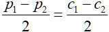
（1）交叉前后两父代与两子代数值的平均值相等，即

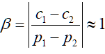
（2）交叉前后两父代差值与两子代差值的商略等于1，即

交叉操作基本过程如下：
（1）在选择操作得到的种群中，随机选择两个个体 ;
（2）生成一个分布随机数 ；
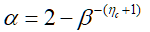
（3）通过多项式概率分布计算参数 ，其计算公式为

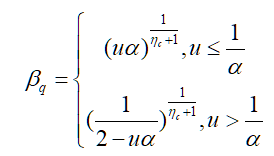
其中，ηc为交叉操作的分布指标，ηc非负数 且值越大代表子代与父代更接近；

（4）计算交叉后子代：

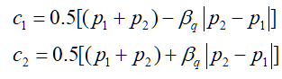
代码如下：

unction child_offspring  = genetic_operator(parent_selected)
global V xl xu etac 
%% Description
% 1. Crossover followed by mutation
% 2. Input is in 'parent_selected' matrix of size [pop_size,V].
% 3. Output is also of same size in 'child_offspring'. 
%% Reference 
% Deb & samir agrawal,"A Niched-Penalty Approach for Constraint Handling in Genetic Algorithms". 
%% SBX cross over operation incorporating boundary constraint
[N] = size(parent_selected,1);
xl1=xl';
xu1=xu';
rc=randperm(N);
for i=1:(N/2)
parent1=parent_selected((rc(2*i-1)),:);
parent2=parent_selected((rc(2*i)),:);
if (isequal(parent1,parent2))==1 & rand(1)>0.5
child1=parent1;
child2=parent2;
else 
for j = 1: V  
if parent1(j)<parent2(j)
beta(j)= 1 + (2/(parent2(j)-parent1(j)))*(min((parent1(j)-xl1(j)),(xu1(j)-parent2(j))));
else
beta(j)= 1 + (2/(parent1(j)-parent2(j)))*(min((parent2(j)-xl1(j)),(xu1(j)-parent1(j))));
end   
end
u=rand(1,V);
alpha=2-beta.^-(etac+1);
betaq=(u<=(1./alpha)).*(u.*alpha).^(1/(etac+1))+(u>(1./alpha)).*(1./(2 - u.*alpha)).^(1/(etac+1));
child1=0.5*(((1 + betaq).*parent1) + (1 - betaq).*parent2);
child2=0.5*(((1 - betaq).*parent1) + (1 + betaq).*parent2);
end
child_offspring((rc(2*i-1)),:)=poly_mutation(child1);           % polynomial mutation
child_offspring((rc(2*i)),:)=poly_mutation(child2);             % polynomial mutation
end

对模拟二进制交叉的简介可以参考：作者 武科大许志伟，标题 模拟二进制交叉算子详解

多项式变异

本例中的变异操作为多项式变异操作，同样由Deb等人在文献[2]中提出。多项式变异的过程为：
（1）生成一个分布随机数u∈[0,1) ；
（2）通过多项式计算参数 ，其中计算公式为：

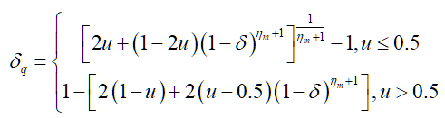
其中

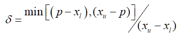
ηm为变异分布指标,ηm越大表示子代离父代越近。
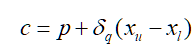
（3）计算变异后子代：

精英保留策略

经过选择、交叉、变异操作后，得到了子代种群 Qi，将父代Pi 与子代 Qi合并成种群 。此处应用精英保留策略产生下一代的父代种群 Ri。首先将合并后的种群Ri进行非支配排序并计算聚集距离，得到等级从低到高排列的分好层的种群，将每层种群放入下一代的父代种群Pi+1中，知道某一层的个体不能全部放入父代种群Pi+1中。那么将该层的个体按照聚集距离由大到小排列，依次放入父代种群Pi+1中，直到Pi+1被填满。
代码如下：

function mutated_child = poly_mutation(y)
global V xl xu etam pm
%% Description
% 1. Input is the crossovered child of size (1,V) in the vector 'y' from 'genetic_operator.m'.
% 2. Output is in the vector 'mutated_child' of size (1,V).
%% Polynomial mutation including boundary constraint
del=min((y-xl),(xu-y))./(xu-xl);
t=rand(1,V);
loc_mut=t<pm;        
u=rand(1,V);
delq=(u<=0.5).*((((2*u)+((1-2*u).*((1-del).^(etam+1)))).^(1/(etam+1)))-1)+(u>0.5).*(1-((2*(1-u))+(2*(u-0.5).*((1-del).^(etam+1)))).^(1/(etam+1)));
c=y+delq.*loc_mut.*(xu-xl);
mutated_child=c;   

参考文献

[1] Meyarivan, T., et al. “A fast and elitist multiobjective genetic algorithm: NSGA-II.” IEEE Trans Evol Comput 6.2 (2002): 182-197.
[2] Deb, Kalyanmoy, and Samir Agrawal. “A niched-penalty approach for constraint handling in genetic algorithms.” Artificial Neural Nets and Genetic Algorithms. Springer, Vienna, 1999.