大家好，又见面了，我是你们的朋友全栈君。

学习前言

也做了一下pytorch版本的。
在这里插入图片描述

什么是YOLOV4

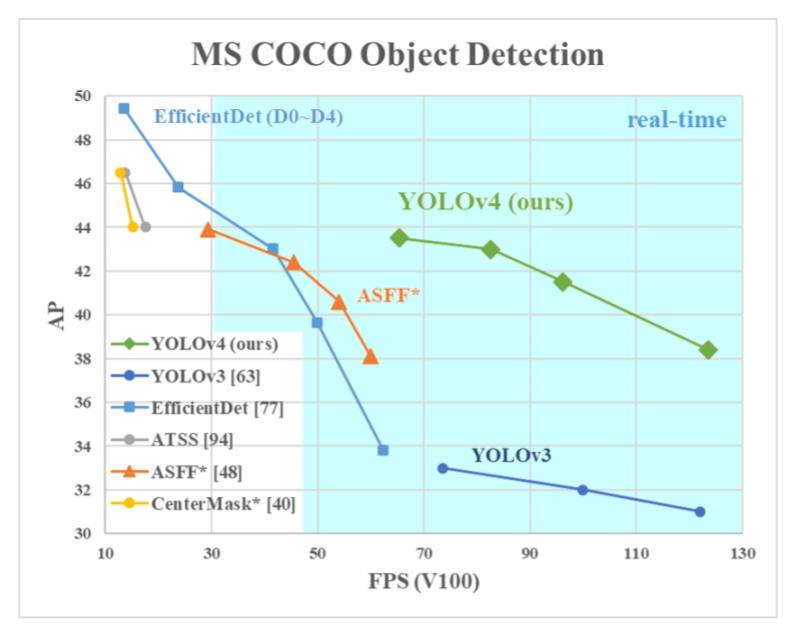
YOLOV4是YOLOV3的改进版，在YOLOV3的基础上结合了非常多的小Tricks。
尽管没有目标检测上革命性的改变，但是YOLOV4依然很好的结合了速度与精度。
根据上图也可以看出来，YOLOV4在YOLOV3的基础上，在FPS不下降的情况下，mAP达到了44，提高非常明显。

YOLOV4整体上的检测思路和YOLOV3相比相差并不大，都是使用三个特征层进行分类与回归预测。

请注意！

强烈建议在学习YOLOV4之前学习YOLOV3，因为YOLOV4确实可以看作是YOLOV3结合一系列改进的版本！

（重要的事情说三遍！）

YOLOV3可参考该博客：
https://blog.csdn.net/weixin_44791964/article/details/105310627

代码下载

https://github.com/bubbliiiing/yolov4-pytorch
喜欢的可以给个star噢！

YOLOV4改进的部分（不完全）

1、主干特征提取网络：DarkNet53 => CSPDarkNet53

2、特征金字塔：SPP，PAN

3、分类回归层：YOLOv3（未改变）

4、训练用到的小技巧：Mosaic数据增强、Label Smoothing平滑、CIOU、学习率余弦退火衰减

5、激活函数：使用Mish激活函数

以上并非全部的改进部分，还存在一些其它的改进，由于YOLOV4使用的改进实在太多了，很难完全实现与列出来，这里只列出来了一些我比较感兴趣，而且非常有效的改进。

还有一个重要的事情：
论文中提到的SAM，作者自己的源码也没有使用。

还有其它很多的tricks，不是所有的tricks都有提升，我也没法实现全部的tricks。

整篇BLOG会结合YOLOV3与YOLOV4的差别进行解析

YOLOV4结构解析

为方便理解，本文将所有通道数都放到了最后一维度。
为方便理解，本文将所有通道数都放到了最后一维度。
为方便理解，本文将所有通道数都放到了最后一维度。

1、主干特征提取网络Backbone

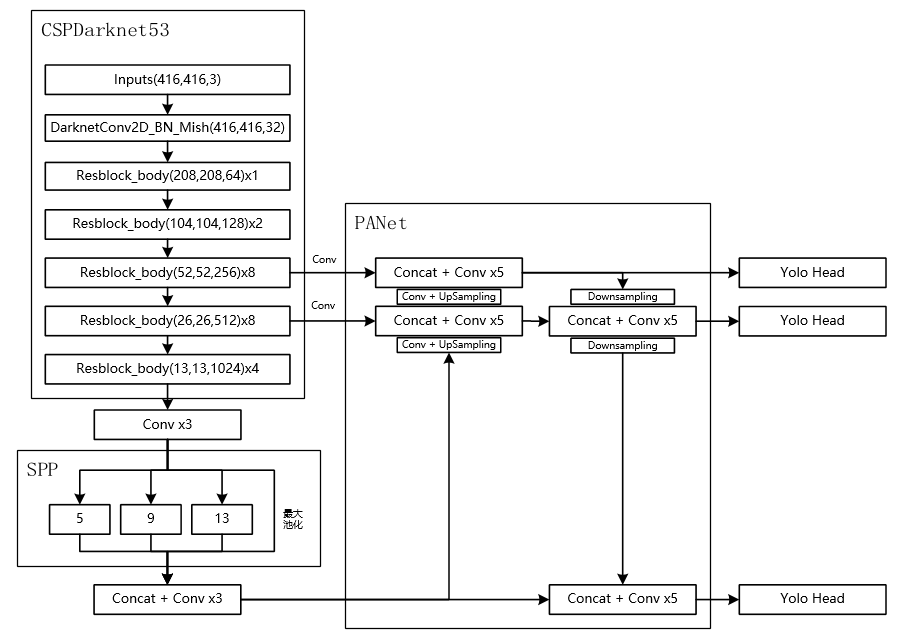
当输入是416×416时，特征结构如下：

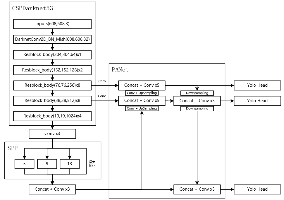
当输入是608×608时，特征结构如下：

主干特征提取网络Backbone的改进点有两个：
a).主干特征提取网络：DarkNet53 => CSPDarkNet53
b).激活函数：使用Mish激活函数

如果大家对YOLOV3比较熟悉的话，应该知道Darknet53的结构，其由一系列残差网络结构构成。在Darknet53中，其存在resblock_body模块，其由一次下采样和多次残差结构的堆叠构成，Darknet53便是由resblock_body模块组合而成。

而在YOLOV4中，其对该部分进行了一定的修改。
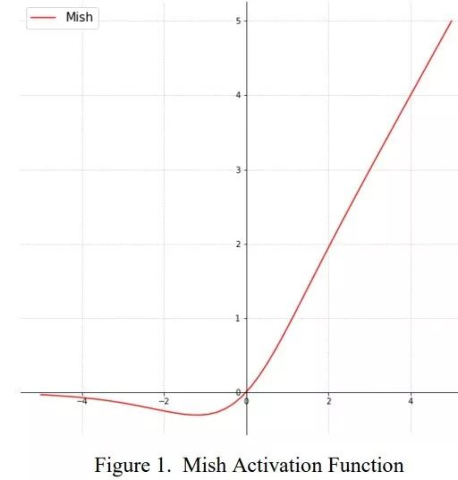
1、其一是将DarknetConv2D的激活函数由LeakyReLU修改成了Mish，卷积块由DarknetConv2D_BN_Leaky变成了DarknetConv2D_BN_Mish。
Mish函数的公式与图像如下：
$\times tanh(ln(1+e^x))$

2、其二是将resblock_body的结构进行修改，使用了CSPnet结构。此时YOLOV4当中的Darknet53被修改成了CSPDarknet53。

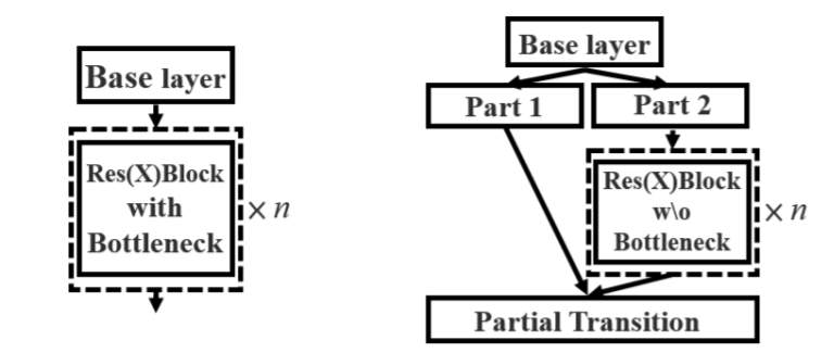
CSPnet结构并不算复杂，就是将原来的残差块的堆叠进行了一个拆分，拆成左右两部分：
主干部分继续进行原来的残差块的堆叠；
另一部分则像一个残差边一样，经过少量处理直接连接到最后。
因此可以认为CSP中存在一个大的残差边。

#---------------------------------------------------#
# CSPdarknet的结构块
# 存在一个大残差边
# 这个大残差边绕过了很多的残差结构
#---------------------------------------------------#
class Resblock_body(nn.Module):
    def __init__(self, in_channels, out_channels, num_blocks, first):
        super(Resblock_body, self).__init__()

        self.downsample_conv = BasicConv(in_channels, out_channels, 3, stride=2)

        if first:
            self.split_conv0 = BasicConv(out_channels, out_channels, 1)
            self.split_conv1 = BasicConv(out_channels, out_channels, 1)  
            self.blocks_conv = nn.Sequential(
                Resblock(channels=out_channels, hidden_channels=out_channels//2),
                BasicConv(out_channels, out_channels, 1)
            )
            self.concat_conv = BasicConv(out_channels*2, out_channels, 1)
        else:
            self.split_conv0 = BasicConv(out_channels, out_channels//2, 1)
            self.split_conv1 = BasicConv(out_channels, out_channels//2, 1)

            self.blocks_conv = nn.Sequential(
                *[Resblock(out_channels//2) for _ in range(num_blocks)],
                BasicConv(out_channels//2, out_channels//2, 1)
            )
            self.concat_conv = BasicConv(out_channels, out_channels, 1)

    def forward(self, x):
        x = self.downsample_conv(x)

        x0 = self.split_conv0(x)

        x1 = self.split_conv1(x)
        x1 = self.blocks_conv(x1)

        x = torch.cat([x1, x0], dim=1)
        x = self.concat_conv(x)

        return x

全部实现代码为：

import torch
import torch.nn.functional as F
import torch.nn as nn
import math
from collections import OrderedDict
#-------------------------------------------------#
# MISH激活函数
#-------------------------------------------------#
class Mish(nn.Module):
def __init__(self):
super(Mish, self).__init__()
def forward(self, x):
return x * torch.tanh(F.softplus(x))
#-------------------------------------------------#
# 卷积块
# CONV+BATCHNORM+MISH
#-------------------------------------------------#
class BasicConv(nn.Module):
def __init__(self, in_channels, out_channels, kernel_size, stride=1):
super(BasicConv, self).__init__()
self.conv = nn.Conv2d(in_channels, out_channels, kernel_size, stride, kernel_size//2, bias=False)
self.bn = nn.BatchNorm2d(out_channels)
self.activation = Mish()
def forward(self, x):
x = self.conv(x)
x = self.bn(x)
x = self.activation(x)
return x
#---------------------------------------------------#
# CSPdarknet的结构块的组成部分
# 内部堆叠的残差块
#---------------------------------------------------#
class Resblock(nn.Module):
def __init__(self, channels, hidden_channels=None, residual_activation=nn.Identity()):
super(Resblock, self).__init__()
if hidden_channels is None:
hidden_channels = channels
self.block = nn.Sequential(
BasicConv(channels, hidden_channels, 1),
BasicConv(hidden_channels, channels, 3)
)
def forward(self, x):
return x+self.block(x)
#---------------------------------------------------#
# CSPdarknet的结构块
# 存在一个大残差边
# 这个大残差边绕过了很多的残差结构
#---------------------------------------------------#
class Resblock_body(nn.Module):
def __init__(self, in_channels, out_channels, num_blocks, first):
super(Resblock_body, self).__init__()
self.downsample_conv = BasicConv(in_channels, out_channels, 3, stride=2)
if first:
self.split_conv0 = BasicConv(out_channels, out_channels, 1)
self.split_conv1 = BasicConv(out_channels, out_channels, 1)  
self.blocks_conv = nn.Sequential(
Resblock(channels=out_channels, hidden_channels=out_channels//2),
BasicConv(out_channels, out_channels, 1)
)
self.concat_conv = BasicConv(out_channels*2, out_channels, 1)
else:
self.split_conv0 = BasicConv(out_channels, out_channels//2, 1)
self.split_conv1 = BasicConv(out_channels, out_channels//2, 1)
self.blocks_conv = nn.Sequential(
*[Resblock(out_channels//2) for _ in range(num_blocks)],
BasicConv(out_channels//2, out_channels//2, 1)
)
self.concat_conv = BasicConv(out_channels, out_channels, 1)
def forward(self, x):
x = self.downsample_conv(x)
x0 = self.split_conv0(x)
x1 = self.split_conv1(x)
x1 = self.blocks_conv(x1)
x = torch.cat([x1, x0], dim=1)
x = self.concat_conv(x)
return x
class CSPDarkNet(nn.Module):
def __init__(self, layers):
super(CSPDarkNet, self).__init__()
self.inplanes = 32
self.conv1 = BasicConv(3, self.inplanes, kernel_size=3, stride=1)
self.feature_channels = [64, 128, 256, 512, 1024]
self.stages = nn.ModuleList([
Resblock_body(self.inplanes, self.feature_channels[0], layers[0], first=True),
Resblock_body(self.feature_channels[0], self.feature_channels[1], layers[1], first=False),
Resblock_body(self.feature_channels[1], self.feature_channels[2], layers[2], first=False),
Resblock_body(self.feature_channels[2], self.feature_channels[3], layers[3], first=False),
Resblock_body(self.feature_channels[3], self.feature_channels[4], layers[4], first=False)
])
self.num_features = 1
# 进行权值初始化
for m in self.modules():
if isinstance(m, nn.Conv2d):
n = m.kernel_size[0] * m.kernel_size[1] * m.out_channels
m.weight.data.normal_(0, math.sqrt(2. / n))
elif isinstance(m, nn.BatchNorm2d):
m.weight.data.fill_(1)
m.bias.data.zero_()
def forward(self, x):
x = self.conv1(x)
x = self.stages[0](x)
x = self.stages[1](x)
out3 = self.stages[2](x)
out4 = self.stages[3](out3)
out5 = self.stages[4](out4)
return out3, out4, out5
def darknet53(pretrained, **kwargs):
model = CSPDarkNet([1, 2, 8, 8, 4])
if pretrained:
if isinstance(pretrained, str):
model.load_state_dict(torch.load(pretrained))
else:
raise Exception("darknet request a pretrained path. got [{}]".format(pretrained))
return model

2、特征金字塔

当输入是416×416时，特征结构如下：

当输入是608×608时，特征结构如下：

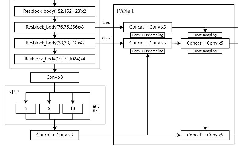
在特征金字塔部分，YOLOV4结合了两种改进:
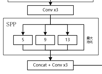
a).使用了SPP结构。
b).使用了PANet结构。
如上图所示，除去CSPDarknet53和Yolo Head的结构外，都是特征金字塔的结构。
1、SPP结构参杂在对CSPdarknet53的最后一个特征层的卷积里，在对CSPdarknet53的最后一个特征层进行三次DarknetConv2D_BN_Leaky卷积后，分别利用四个不同尺度的最大池化进行处理，最大池化的池化核大小分别为13×13、9×9、5×5、1×1（1×1即无处理）

#---------------------------------------------------#
# SPP结构，利用不同大小的池化核进行池化
# 池化后堆叠
#---------------------------------------------------#
class SpatialPyramidPooling(nn.Module):
def __init__(self, pool_sizes=[5, 9, 13]):
super(SpatialPyramidPooling, self).__init__()
self.maxpools = nn.ModuleList([nn.MaxPool2d(pool_size, 1, pool_size//2) for pool_size in pool_sizes])
def forward(self, x):
features = [maxpool(x) for maxpool in self.maxpools[::-1]]
features = torch.cat(features + [x], dim=1)
return features

其可以它能够极大地增加感受野，分离出最显著的上下文特征。

2、PANet是2018的一种实例分割算法，其具体结构由反复提升特征的意思。

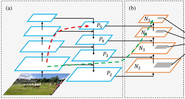
上图为原始的PANet的结构，可以看出来其具有一个非常重要的特点就是特征的反复提取。
在（a）里面是传统的特征金字塔结构，在完成特征金字塔从下到上的特征提取后，还需要实现（b）中从上到下的特征提取。

而在YOLOV4当中，其主要是在三个有效特征层上使用了PANet结构。

实现代码如下：

#---------------------------------------------------#
# yolo_body
#---------------------------------------------------#
class YoloBody(nn.Module):
def __init__(self, config):
super(YoloBody, self).__init__()
self.config = config
# backbone
self.backbone = darknet53(None)
self.conv1 = make_three_conv([512,1024],1024)
self.SPP = SpatialPyramidPooling()
self.conv2 = make_three_conv([512,1024],2048)
self.upsample1 = Upsample(512,256)
self.conv_for_P4 = conv2d(512,256,1)
self.make_five_conv1 = make_five_conv([256, 512],512)
self.upsample2 = Upsample(256,128)
self.conv_for_P3 = conv2d(256,128,1)
self.make_five_conv2 = make_five_conv([128, 256],256)
# 3*(5+num_classes)=3*(5+20)=3*(4+1+20)=75
final_out_filter2 = len(config["yolo"]["anchors"][2]) * (5 + config["yolo"]["classes"])
self.yolo_head3 = yolo_head([256, final_out_filter2],128)
self.down_sample1 = conv2d(128,256,3,stride=2)
self.make_five_conv3 = make_five_conv([256, 512],512)
# 3*(5+num_classes)=3*(5+20)=3*(4+1+20)=75
final_out_filter1 = len(config["yolo"]["anchors"][1]) * (5 + config["yolo"]["classes"])
self.yolo_head2 = yolo_head([512, final_out_filter1],256)
self.down_sample2 = conv2d(256,512,3,stride=2)
self.make_five_conv4 = make_five_conv([512, 1024],1024)
# 3*(5+num_classes)=3*(5+20)=3*(4+1+20)=75
final_out_filter0 = len(config["yolo"]["anchors"][0]) * (5 + config["yolo"]["classes"])
self.yolo_head1 = yolo_head([1024, final_out_filter0],512)
def forward(self, x):
# backbone
x2, x1, x0 = self.backbone(x)
P5 = self.conv1(x0)
P5 = self.SPP(P5)
P5 = self.conv2(P5)
P5_upsample = self.upsample1(P5)
P4 = self.conv_for_P4(x1)
P4 = torch.cat([P4,P5_upsample],axis=1)
P4 = self.make_five_conv1(P4)
P4_upsample = self.upsample2(P4)
P3 = self.conv_for_P3(x2)
P3 = torch.cat([P3,P4_upsample],axis=1)
P3 = self.make_five_conv2(P3)
P3_downsample = self.down_sample1(P3)
P4 = torch.cat([P3_downsample,P4],axis=1)
P4 = self.make_five_conv3(P4)
P4_downsample = self.down_sample2(P4)
P5 = torch.cat([P4_downsample,P5],axis=1)
P5 = self.make_five_conv4(P5)
out2 = self.yolo_head3(P3)
out1 = self.yolo_head2(P4)
out0 = self.yolo_head1(P5)
return out0, out1, out2

3、YoloHead利用获得到的特征进行预测

当输入是416×416时，特征结构如下：

当输入是608×608时，特征结构如下：

1、在特征利用部分，YoloV4提取多特征层进行目标检测，一共提取三个特征层，分别位于中间层，中下层，底层，三个特征层的shape分别为(76,76,256)、(38,38,512)、(19,19,1024)。

2、输出层的shape分别为(19,19,75)，(38,38,75)，(76,76,75)，最后一个维度为75是因为该图是基于voc数据集的，它的类为20种，YoloV4只有针对每一个特征层存在3个先验框，所以最后维度为3×25；
如果使用的是coco训练集，类则为80种，最后的维度应该为255 = 3×85，三个特征层的shape为(19,19,255)，(38,38,255)，(76,76,255)

实现代码如下：

#---------------------------------------------------#
# 最后获得yolov4的输出
#---------------------------------------------------#
def yolo_head(filters_list, in_filters):
m = nn.Sequential(
conv2d(in_filters, filters_list[0], 3),
nn.Conv2d(filters_list[0], filters_list[1], 1),
)
return m
#---------------------------------------------------#
# yolo_body
#---------------------------------------------------#
class YoloBody(nn.Module):
def __init__(self, config):
super(YoloBody, self).__init__()
self.config = config
# backbone
self.backbone = darknet53(None)
self.conv1 = make_three_conv([512,1024],1024)
self.SPP = SpatialPyramidPooling()
self.conv2 = make_three_conv([512,1024],2048)
self.upsample1 = Upsample(512,256)
self.conv_for_P4 = conv2d(512,256,1)
self.make_five_conv1 = make_five_conv([256, 512],512)
self.upsample2 = Upsample(256,128)
self.conv_for_P3 = conv2d(256,128,1)
self.make_five_conv2 = make_five_conv([128, 256],256)
# 3*(5+num_classes)=3*(5+20)=3*(4+1+20)=75
final_out_filter2 = len(config["yolo"]["anchors"][2]) * (5 + config["yolo"]["classes"])
self.yolo_head3 = yolo_head([256, final_out_filter2],128)
self.down_sample1 = conv2d(128,256,3,stride=2)
self.make_five_conv3 = make_five_conv([256, 512],512)
# 3*(5+num_classes)=3*(5+20)=3*(4+1+20)=75
final_out_filter1 = len(config["yolo"]["anchors"][1]) * (5 + config["yolo"]["classes"])
self.yolo_head2 = yolo_head([512, final_out_filter1],256)
self.down_sample2 = conv2d(256,512,3,stride=2)
self.make_five_conv4 = make_five_conv([512, 1024],1024)
# 3*(5+num_classes)=3*(5+20)=3*(4+1+20)=75
final_out_filter0 = len(config["yolo"]["anchors"][0]) * (5 + config["yolo"]["classes"])
self.yolo_head1 = yolo_head([1024, final_out_filter0],512)
def forward(self, x):
# backbone
x2, x1, x0 = self.backbone(x)
P5 = self.conv1(x0)
P5 = self.SPP(P5)
P5 = self.conv2(P5)
P5_upsample = self.upsample1(P5)
P4 = self.conv_for_P4(x1)
P4 = torch.cat([P4,P5_upsample],axis=1)
P4 = self.make_five_conv1(P4)
P4_upsample = self.upsample2(P4)
P3 = self.conv_for_P3(x2)
P3 = torch.cat([P3,P4_upsample],axis=1)
P3 = self.make_five_conv2(P3)
P3_downsample = self.down_sample1(P3)
P4 = torch.cat([P3_downsample,P4],axis=1)
P4 = self.make_five_conv3(P4)
P4_downsample = self.down_sample2(P4)
P5 = torch.cat([P4_downsample,P5],axis=1)
P5 = self.make_five_conv4(P5)
out2 = self.yolo_head3(P3)
out1 = self.yolo_head2(P4)
out0 = self.yolo_head1(P5)
return out0, out1, out2

4、预测结果的解码

由第二步我们可以获得三个特征层的预测结果，shape分别为(N,19,19,255)，(N,38,38,255)，(N,76,76,255)的数据，对应每个图分为19×19、38×38、76×76的网格上3个预测框的位置。

但是这个预测结果并不对应着最终的预测框在图片上的位置，还需要解码才可以完成。

此处要讲一下yolo3的预测原理，yolo3的3个特征层分别将整幅图分为19×19、38×38、76×76的网格，每个网络点负责一个区域的检测。

我们知道特征层的预测结果对应着三个预测框的位置，我们先将其reshape一下，其结果为(N,19,19,3,85)，(N,38,38,3,85)，(N,76,76,3,85)。

最后一个维度中的85包含了4+1+80，分别代表x_offset、y_offset、h和w、置信度、分类结果。

yolo3的解码过程就是将每个网格点加上它对应的x_offset和y_offset，加完后的结果就是预测框的中心，然后再利用先验框和h、w结合计算出预测框的长和宽。这样就能得到整个预测框的位置了。

当然得到最终的预测结构后还要进行得分排序与非极大抑制筛选
这一部分基本上是所有目标检测通用的部分。不过该项目的处理方式与其它项目不同。其对于每一个类进行判别。
1、取出每一类得分大于self.obj_threshold的框和得分。
2、利用框的位置和得分进行非极大抑制。

实现代码如下，当调用yolo_eval时，就会对每个特征层进行解码：

import torch
import torch.nn as nn
from torchvision.ops import nms
import numpy as np
class DecodeBox():
def __init__(self, anchors, num_classes, input_shape, anchors_mask = [[6,7,8], [3,4,5], [0,1,2]]):
super(DecodeBox, self).__init__()
self.anchors        = anchors
self.num_classes    = num_classes
self.bbox_attrs     = 5 + num_classes
self.input_shape    = input_shape
#-----------------------------------------------------------#
# 13x13的特征层对应的anchor是[142, 110],[192, 243],[459, 401]
# 26x26的特征层对应的anchor是[36, 75],[76, 55],[72, 146]
# 52x52的特征层对应的anchor是[12, 16],[19, 36],[40, 28]
#-----------------------------------------------------------#
self.anchors_mask   = anchors_mask
def decode_box(self, inputs):
outputs = []
for i, input in enumerate(inputs):
#-----------------------------------------------#
# 输入的input一共有三个，他们的shape分别是
# batch_size, 255, 13, 13
# batch_size, 255, 26, 26
# batch_size, 255, 52, 52
#-----------------------------------------------#
batch_size      = input.size(0)
input_height    = input.size(2)
input_width     = input.size(3)
#-----------------------------------------------#
# 输入为416x416时
# stride_h = stride_w = 32、16、8
#-----------------------------------------------#
stride_h = self.input_shape[0] / input_height
stride_w = self.input_shape[1] / input_width
#-------------------------------------------------#
# 此时获得的scaled_anchors大小是相对于特征层的
#-------------------------------------------------#
scaled_anchors = [(anchor_width / stride_w, anchor_height / stride_h) for anchor_width, anchor_height in self.anchors[self.anchors_mask[i]]]
#-----------------------------------------------#
# 输入的input一共有三个，他们的shape分别是
# batch_size, 3, 13, 13, 85
# batch_size, 3, 26, 26, 85
# batch_size, 3, 52, 52, 85
#-----------------------------------------------#
prediction = input.view(batch_size, len(self.anchors_mask[i]),
self.bbox_attrs, input_height, input_width).permute(0, 1, 3, 4, 2).contiguous()
#-----------------------------------------------#
# 先验框的中心位置的调整参数
#-----------------------------------------------#
x = torch.sigmoid(prediction[..., 0])  
y = torch.sigmoid(prediction[..., 1])
#-----------------------------------------------#
# 先验框的宽高调整参数
#-----------------------------------------------#
w = prediction[..., 2]
h = prediction[..., 3]
#-----------------------------------------------#
# 获得置信度，是否有物体
#-----------------------------------------------#
conf        = torch.sigmoid(prediction[..., 4])
#-----------------------------------------------#
# 种类置信度
#-----------------------------------------------#
pred_cls    = torch.sigmoid(prediction[..., 5:])
FloatTensor = torch.cuda.FloatTensor if x.is_cuda else torch.FloatTensor
LongTensor  = torch.cuda.LongTensor if x.is_cuda else torch.LongTensor
#----------------------------------------------------------#
# 生成网格，先验框中心，网格左上角 
# batch_size,3,13,13
#----------------------------------------------------------#
grid_x = torch.linspace(0, input_width - 1, input_width).repeat(input_height, 1).repeat(
batch_size * len(self.anchors_mask[i]), 1, 1).view(x.shape).type(FloatTensor)
grid_y = torch.linspace(0, input_height - 1, input_height).repeat(input_width, 1).t().repeat(
batch_size * len(self.anchors_mask[i]), 1, 1).view(y.shape).type(FloatTensor)
#----------------------------------------------------------#
# 按照网格格式生成先验框的宽高
# batch_size,3,13,13
#----------------------------------------------------------#
anchor_w = FloatTensor(scaled_anchors).index_select(1, LongTensor([0]))
anchor_h = FloatTensor(scaled_anchors).index_select(1, LongTensor([1]))
anchor_w = anchor_w.repeat(batch_size, 1).repeat(1, 1, input_height * input_width).view(w.shape)
anchor_h = anchor_h.repeat(batch_size, 1).repeat(1, 1, input_height * input_width).view(h.shape)
#----------------------------------------------------------#
# 利用预测结果对先验框进行调整
# 首先调整先验框的中心，从先验框中心向右下角偏移
# 再调整先验框的宽高。
#----------------------------------------------------------#
pred_boxes          = FloatTensor(prediction[..., :4].shape)
pred_boxes[..., 0]  = x.data + grid_x
pred_boxes[..., 1]  = y.data + grid_y
pred_boxes[..., 2]  = torch.exp(w.data) * anchor_w
pred_boxes[..., 3]  = torch.exp(h.data) * anchor_h
#----------------------------------------------------------#
# 将输出结果归一化成小数的形式
#----------------------------------------------------------#
_scale = torch.Tensor([input_width, input_height, input_width, input_height]).type(FloatTensor)
output = torch.cat((pred_boxes.view(batch_size, -1, 4) / _scale,
conf.view(batch_size, -1, 1), pred_cls.view(batch_size, -1, self.num_classes)), -1)
outputs.append(output.data)
return outputs
def yolo_correct_boxes(self, box_xy, box_wh, input_shape, image_shape, letterbox_image):
#-----------------------------------------------------------------#
# 把y轴放前面是因为方便预测框和图像的宽高进行相乘
#-----------------------------------------------------------------#
box_yx = box_xy[..., ::-1]
box_hw = box_wh[..., ::-1]
input_shape = np.array(input_shape)
image_shape = np.array(image_shape)
if letterbox_image:
#-----------------------------------------------------------------#
# 这里求出来的offset是图像有效区域相对于图像左上角的偏移情况
# new_shape指的是宽高缩放情况
#-----------------------------------------------------------------#
new_shape = np.round(image_shape * np.min(input_shape/image_shape))
offset  = (input_shape - new_shape)/2./input_shape
scale   = input_shape/new_shape
box_yx  = (box_yx - offset) * scale
box_hw *= scale
box_mins    = box_yx - (box_hw / 2.)
box_maxes   = box_yx + (box_hw / 2.)
boxes  = np.concatenate([box_mins[..., 0:1], box_mins[..., 1:2], box_maxes[..., 0:1], box_maxes[..., 1:2]], axis=-1)
boxes *= np.concatenate([image_shape, image_shape], axis=-1)
return boxes
def non_max_suppression(self, prediction, num_classes, input_shape, image_shape, letterbox_image, conf_thres=0.5, nms_thres=0.4):
#----------------------------------------------------------#
# 将预测结果的格式转换成左上角右下角的格式。
# prediction [batch_size, num_anchors, 85]
#----------------------------------------------------------#
box_corner          = prediction.new(prediction.shape)
box_corner[:, :, 0] = prediction[:, :, 0] - prediction[:, :, 2] / 2
box_corner[:, :, 1] = prediction[:, :, 1] - prediction[:, :, 3] / 2
box_corner[:, :, 2] = prediction[:, :, 0] + prediction[:, :, 2] / 2
box_corner[:, :, 3] = prediction[:, :, 1] + prediction[:, :, 3] / 2
prediction[:, :, :4] = box_corner[:, :, :4]
output = [None for _ in range(len(prediction))]
for i, image_pred in enumerate(prediction):
#----------------------------------------------------------#
# 对种类预测部分取max。
# class_conf [num_anchors, 1] 种类置信度
# class_pred [num_anchors, 1] 种类
#----------------------------------------------------------#
class_conf, class_pred = torch.max(image_pred[:, 5:5 + num_classes], 1, keepdim=True)
#----------------------------------------------------------#
# 利用置信度进行第一轮筛选
#----------------------------------------------------------#
conf_mask = (image_pred[:, 4] * class_conf[:, 0] >= conf_thres).squeeze()
#----------------------------------------------------------#
# 根据置信度进行预测结果的筛选
#----------------------------------------------------------#
image_pred = image_pred[conf_mask]
class_conf = class_conf[conf_mask]
class_pred = class_pred[conf_mask]
if not image_pred.size(0):
continue
#-------------------------------------------------------------------------#
# detections [num_anchors, 7]
# 7的内容为：x1, y1, x2, y2, obj_conf, class_conf, class_pred
#-------------------------------------------------------------------------#
detections = torch.cat((image_pred[:, :5], class_conf.float(), class_pred.float()), 1)
#------------------------------------------#
# 获得预测结果中包含的所有种类
#------------------------------------------#
unique_labels = detections[:, -1].cpu().unique()
if prediction.is_cuda:
unique_labels = unique_labels.cuda()
detections = detections.cuda()
for c in unique_labels:
#------------------------------------------#
# 获得某一类得分筛选后全部的预测结果
#------------------------------------------#
detections_class = detections[detections[:, -1] == c]
#------------------------------------------#
# 使用官方自带的非极大抑制会速度更快一些！
#------------------------------------------#
keep = nms(
detections_class[:, :4],
detections_class[:, 4] * detections_class[:, 5],
nms_thres
)
max_detections = detections_class[keep]
# # 按照存在物体的置信度排序
# _, conf_sort_index = torch.sort(detections_class[:, 4]*detections_class[:, 5], descending=True)
# detections_class = detections_class[conf_sort_index]
# # 进行非极大抑制
# max_detections = []
# while detections_class.size(0):
# # 取出这一类置信度最高的，一步一步往下判断，判断重合程度是否大于nms_thres，如果是则去除掉
# max_detections.append(detections_class[0].unsqueeze(0))
# if len(detections_class) == 1:
# break
# ious = bbox_iou(max_detections[-1], detections_class[1:])
# detections_class = detections_class[1:][ious < nms_thres]
# # 堆叠
# max_detections = torch.cat(max_detections).data
# Add max detections to outputs
output[i] = max_detections if output[i] is None else torch.cat((output[i], max_detections))
if output[i] is not None:
output[i]           = output[i].cpu().numpy()
box_xy, box_wh      = (output[i][:, 0:2] + output[i][:, 2:4])/2, output[i][:, 2:4] - output[i][:, 0:2]
output[i][:, :4]    = self.yolo_correct_boxes(box_xy, box_wh, input_shape, image_shape, letterbox_image)
return output

5、在原图上进行绘制

通过第四步，我们可以获得预测框在原图上的位置，而且这些预测框都是经过筛选的。这些筛选后的框可以直接绘制在图片上，就可以获得结果了。

YOLOV4的训练

1、YOLOV4的改进训练技巧

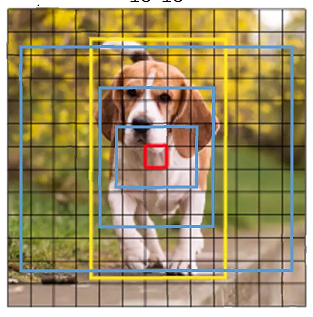
a)、Mosaic数据增强

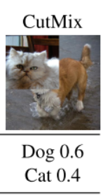
Yolov4的mosaic数据增强参考了CutMix数据增强方式，理论上具有一定的相似性！
CutMix数据增强方式利用两张图片进行拼接。

但是mosaic利用了四张图片，根据论文所说其拥有一个巨大的优点是丰富检测物体的背景！且在BN计算的时候一下子会计算四张图片的数据！
就像下图这样：

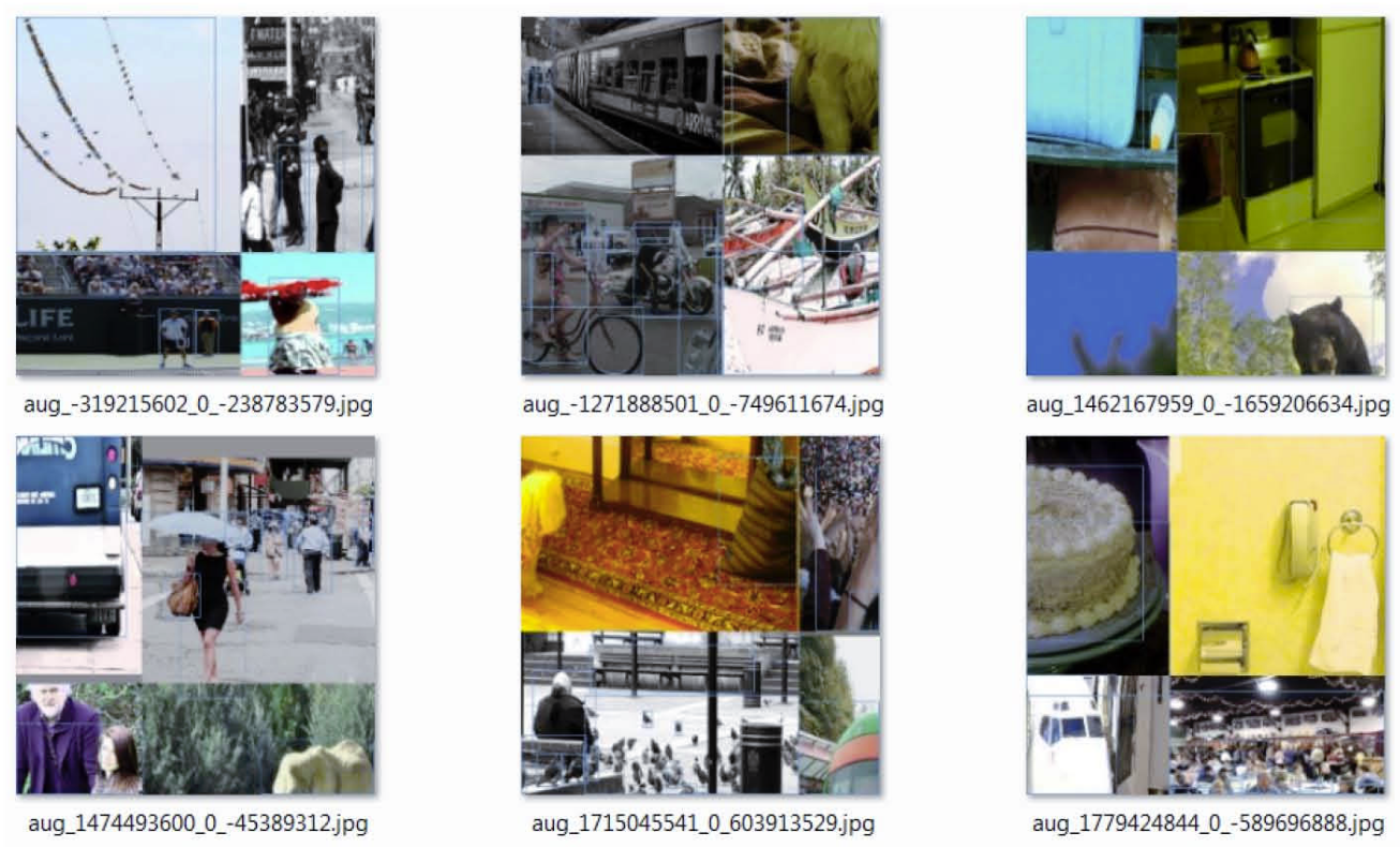
实现思路如下：
1、每次读取四张图片。

2、分别对四张图片进行翻转、缩放、色域变化等，并且按照四个方向位置摆好。

3、进行图片的组合和框的组合

def merge_bboxes(self, bboxes, cutx, cuty):
merge_bbox = []
for i in range(len(bboxes)):
for box in bboxes[i]:
tmp_box = []
x1, y1, x2, y2 = box[0], box[1], box[2], box[3]
if i == 0:
if y1 > cuty or x1 > cutx:
continue
if y2 >= cuty and y1 <= cuty:
y2 = cuty
if x2 >= cutx and x1 <= cutx:
x2 = cutx
if i == 1:
if y2 < cuty or x1 > cutx:
continue
if y2 >= cuty and y1 <= cuty:
y1 = cuty
if x2 >= cutx and x1 <= cutx:
x2 = cutx
if i == 2:
if y2 < cuty or x2 < cutx:
continue
if y2 >= cuty and y1 <= cuty:
y1 = cuty
if x2 >= cutx and x1 <= cutx:
x1 = cutx
if i == 3:
if y1 > cuty or x2 < cutx:
continue
if y2 >= cuty and y1 <= cuty:
y2 = cuty
if x2 >= cutx and x1 <= cutx:
x1 = cutx
tmp_box.append(x1)
tmp_box.append(y1)
tmp_box.append(x2)
tmp_box.append(y2)
tmp_box.append(box[-1])
merge_bbox.append(tmp_box)
return merge_bbox
def get_random_data_with_Mosaic(self, annotation_line, input_shape, max_boxes=100, hue=.1, sat=1.5, val=1.5):
h, w = input_shape
min_offset_x = self.rand(0.25, 0.75)
min_offset_y = self.rand(0.25, 0.75)
nws     = [ int(w * self.rand(0.4, 1)), int(w * self.rand(0.4, 1)), int(w * self.rand(0.4, 1)), int(w * self.rand(0.4, 1))]
nhs     = [ int(h * self.rand(0.4, 1)), int(h * self.rand(0.4, 1)), int(h * self.rand(0.4, 1)), int(h * self.rand(0.4, 1))]
place_x = [int(w*min_offset_x) - nws[0], int(w*min_offset_x) - nws[1], int(w*min_offset_x), int(w*min_offset_x)]
place_y = [int(h*min_offset_y) - nhs[0], int(h*min_offset_y), int(h*min_offset_y), int(h*min_offset_y) - nhs[3]]
image_datas = [] 
box_datas   = []
index       = 0
for line in annotation_line:
# 每一行进行分割
line_content = line.split()
# 打开图片
image = Image.open(line_content[0])
image = cvtColor(image)
# 图片的大小
iw, ih = image.size
# 保存框的位置
box = np.array([np.array(list(map(int,box.split(',')))) for box in line_content[1:]])
# 是否翻转图片
flip = self.rand()<.5
if flip and len(box)>0:
image = image.transpose(Image.FLIP_LEFT_RIGHT)
box[:, [0,2]] = iw - box[:, [2,0]]
nw = nws[index] 
nh = nhs[index] 
image = image.resize((nw,nh), Image.BICUBIC)
# 将图片进行放置，分别对应四张分割图片的位置
dx = place_x[index]
dy = place_y[index]
new_image = Image.new('RGB', (w,h), (128,128,128))
new_image.paste(image, (dx, dy))
image_data = np.array(new_image)
index = index + 1
box_data = []
# 对box进行重新处理
if len(box)>0:
np.random.shuffle(box)
box[:, [0,2]] = box[:, [0,2]]*nw/iw + dx
box[:, [1,3]] = box[:, [1,3]]*nh/ih + dy
box[:, 0:2][box[:, 0:2]<0] = 0
box[:, 2][box[:, 2]>w] = w
box[:, 3][box[:, 3]>h] = h
box_w = box[:, 2] - box[:, 0]
box_h = box[:, 3] - box[:, 1]
box = box[np.logical_and(box_w>1, box_h>1)]
box_data = np.zeros((len(box),5))
box_data[:len(box)] = box
image_datas.append(image_data)
box_datas.append(box_data)
# 将图片分割，放在一起
cutx = int(w * min_offset_x)
cuty = int(h * min_offset_y)
new_image = np.zeros([h, w, 3])
new_image[:cuty, :cutx, :] = image_datas[0][:cuty, :cutx, :]
new_image[cuty:, :cutx, :] = image_datas[1][cuty:, :cutx, :]
new_image[cuty:, cutx:, :] = image_datas[2][cuty:, cutx:, :]
new_image[:cuty, cutx:, :] = image_datas[3][:cuty, cutx:, :]
# 进行色域变换
hue = self.rand(-hue, hue)
sat = self.rand(1, sat) if self.rand()<.5 else 1/self.rand(1, sat)
val = self.rand(1, val) if self.rand()<.5 else 1/self.rand(1, val)
x = cv2.cvtColor(np.array(new_image/255,np.float32), cv2.COLOR_RGB2HSV)
x[..., 0] += hue*360
x[..., 0][x[..., 0]>1] -= 1
x[..., 0][x[..., 0]<0] += 1
x[..., 1] *= sat
x[..., 2] *= val
x[x[:, :, 0]>360, 0] = 360
x[:, :, 1:][x[:, :, 1:]>1] = 1
x[x<0] = 0
new_image = cv2.cvtColor(x, cv2.COLOR_HSV2RGB)*255
# 对框进行进一步的处理
new_boxes = self.merge_bboxes(box_datas, cutx, cuty)
return new_image, new_boxes

b)、Label Smoothing平滑

标签平滑的思想很简单，具体公式如下：

new_onehot_labels = onehot_labels * (1 - label_smoothing) + label_smoothing / num_classes

当label_smoothing的值为0.01得时候，公式变成如下所示：

new_onehot_labels = y * (1 - 0.01) + 0.01 / num_classes

其实Label Smoothing平滑就是将标签进行一个平滑，原始的标签是0、1，在平滑后变成0.005(如果是二分类)、0.995，也就是说对分类准确做了一点惩罚，让模型不可以分类的太准确，太准确容易过拟合。

实现代码如下：

#---------------------------------------------------#
# 平滑标签
#---------------------------------------------------#
def smooth_labels(y_true, label_smoothing,num_classes):
return y_true * (1.0 - label_smoothing) + label_smoothing / num_classes

c)、CIOU

IoU是比值的概念，对目标物体的scale是不敏感的。然而常用的BBox的回归损失优化和IoU优化不是完全等价的，寻常的IoU无法直接优化没有重叠的部分。

于是有人提出直接使用IOU作为回归优化loss，CIOU是其中非常优秀的一种想法。

CIOU将目标与anchor之间的距离，重叠率、尺度以及惩罚项都考虑进去，使得目标框回归变得更加稳定，不会像IoU和GIoU一样出现训练过程中发散等问题。而惩罚因子把预测框长宽比拟合目标框的长宽比考虑进去。

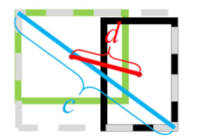
CIOU公式如下
$\frac{\rho^2(b,b^{gt})}{c^2} – \alpha v$
其中， $\rho^2(b,b^{gt})$ 分别代表了预测框和真实框的中心点的欧式距离。 c代表的是能够同时包含预测框和真实框的最小闭包区域的对角线距离。

而 $\alpha$ 和 $v$ 的公式如下
$\alpha = \frac{v}{1-IOU+v}$
$\frac{4}{\pi ^2}(arctan\frac{w^{gt}}{h^{gt}}-arctan\frac{w}{h})^2$
把1-CIOU就可以得到相应的LOSS了。
$LOSS_{CIOU} = 1 – IOU + \frac{\rho^2(b,b^{gt})}{c^2} + \alpha v$

def box_ciou(self, b1, b2):
""" 输入为： ---------- b1: tensor, shape=(batch, feat_w, feat_h, anchor_num, 4), xywh b2: tensor, shape=(batch, feat_w, feat_h, anchor_num, 4), xywh 返回为： ------- ciou: tensor, shape=(batch, feat_w, feat_h, anchor_num, 1) """
#----------------------------------------------------#
# 求出预测框左上角右下角
#----------------------------------------------------#
b1_xy       = b1[..., :2]
b1_wh       = b1[..., 2:4]
b1_wh_half  = b1_wh/2.
b1_mins     = b1_xy - b1_wh_half
b1_maxes    = b1_xy + b1_wh_half
#----------------------------------------------------#
# 求出真实框左上角右下角
#----------------------------------------------------#
b2_xy       = b2[..., :2]
b2_wh       = b2[..., 2:4]
b2_wh_half  = b2_wh/2.
b2_mins     = b2_xy - b2_wh_half
b2_maxes    = b2_xy + b2_wh_half
#----------------------------------------------------#
# 求真实框和预测框所有的iou
#----------------------------------------------------#
intersect_mins  = torch.max(b1_mins, b2_mins)
intersect_maxes = torch.min(b1_maxes, b2_maxes)
intersect_wh    = torch.max(intersect_maxes - intersect_mins, torch.zeros_like(intersect_maxes))
intersect_area  = intersect_wh[..., 0] * intersect_wh[..., 1]
b1_area         = b1_wh[..., 0] * b1_wh[..., 1]
b2_area         = b2_wh[..., 0] * b2_wh[..., 1]
union_area      = b1_area + b2_area - intersect_area
iou             = intersect_area / torch.clamp(union_area,min = 1e-6)
#----------------------------------------------------#
# 计算中心的差距
#----------------------------------------------------#
center_distance = torch.sum(torch.pow((b1_xy - b2_xy), 2), axis=-1)
#----------------------------------------------------#
# 找到包裹两个框的最小框的左上角和右下角
#----------------------------------------------------#
enclose_mins    = torch.min(b1_mins, b2_mins)
enclose_maxes   = torch.max(b1_maxes, b2_maxes)
enclose_wh      = torch.max(enclose_maxes - enclose_mins, torch.zeros_like(intersect_maxes))
#----------------------------------------------------#
# 计算对角线距离
#----------------------------------------------------#
enclose_diagonal = torch.sum(torch.pow(enclose_wh,2), axis=-1)
ciou            = iou - 1.0 * (center_distance) / torch.clamp(enclose_diagonal,min = 1e-6)
v       = (4 / (math.pi ** 2)) * torch.pow((torch.atan(b1_wh[..., 0] / torch.clamp(b1_wh[..., 1],min = 1e-6)) - torch.atan(b2_wh[..., 0] / torch.clamp(b2_wh[..., 1], min = 1e-6))), 2)
alpha   = v / torch.clamp((1.0 - iou + v), min=1e-6)
ciou    = ciou - alpha * v
return ciou

d)、学习率余弦退火衰减

余弦退火衰减法，学习率会先上升再下降，这是退火优化法的思想。（关于什么是退火算法可以百度。）

上升的时候使用线性上升，下降的时候模拟cos函数下降。执行多次。

效果如图所示：

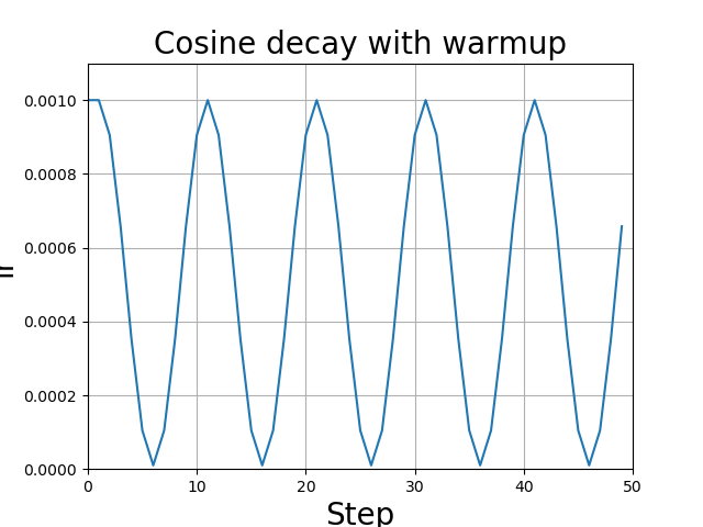
pytorch有直接实现的函数，可直接调用。

lr_scheduler = optim.lr_scheduler.CosineAnnealingLR(optimizer, T_max=5, eta_min=1e-5)

2、loss组成

a)、计算loss所需参数

在计算loss的时候，实际上是y_pre和y_true之间的对比：
y_pre就是一幅图像经过网络之后的输出，内部含有三个特征层的内容；其需要解码才能够在图上作画
y_true就是一个真实图像中，它的每个真实框对应的(19,19)、(38,38)、(76,76)网格上的偏移位置、长宽与种类。其仍需要编码才能与y_pred的结构一致
实际上y_pre和y_true内容的shape都是
(batch_size,19,19,3,85)
(batch_size,38,38,3,85)
(batch_size,76,76,3,85)

b)、y_pre是什么

网络最后输出的内容就是三个特征层每个网格点对应的预测框及其种类，即三个特征层分别对应着图片被分为不同size的网格后，每个网格点上三个先验框对应的位置、置信度及其种类。
对于输出的y1、y2、y3而言，[…, : 2]指的是相对于每个网格点的偏移量，[…, 2: 4]指的是宽和高，[…, 4: 5]指的是该框的置信度，[…, 5: ]指的是每个种类的预测概率。
现在的y_pre还是没有解码的，解码了之后才是真实图像上的情况。

c)、y_true是什么。

y_true就是一个真实图像中，它的每个真实框对应的(19,19)、(38,38)、(76,76)网格上的偏移位置、长宽与种类。其仍需要编码才能与y_pred的结构一致

d)、loss的计算过程

在得到了y_pre和y_true后怎么对比呢？不是简单的减一下!

loss值需要对三个特征层进行处理，这里以最小的特征层为例。
1、利用y_true取出该特征层中真实存在目标的点的位置(m,19,19,3,1)及其对应的种类(m,19,19,3,80)。
2、将prediction的预测值输出进行处理，得到reshape后的预测值y_pre，shape为(m,19,19,3,85)。还有解码后的xy，wh。
3、对于每一幅图，计算其中所有真实框与预测框的IOU，如果某些预测框和真实框的重合程度大于0.5，则忽略。
4、计算ciou作为回归的loss，这里只计算正样本的回归loss。
5、计算置信度的loss，其有两部分构成，第一部分是实际上存在目标的，预测结果中置信度的值与1对比；第二部分是实际上不存在目标的，在第四步中得到其最大IOU的值与0对比。
6、计算预测种类的loss，其计算的是实际上存在目标的，预测类与真实类的差距。

其实际上计算的总的loss是三个loss的和，这三个loss分别是：

实际存在的框，CIOU LOSS。
实际存在的框，预测结果中置信度的值与1对比；实际不存在的框，预测结果中置信度的值与0对比，该部分要去除被忽略的不包含目标的框。
实际存在的框，种类预测结果与实际结果的对比。

其实际代码如下：

import torch
import torch.nn as nn
import math
import numpy as np
class YOLOLoss(nn.Module):
def __init__(self, anchors, num_classes, input_shape, cuda, anchors_mask = [[6,7,8], [3,4,5], [0,1,2]], label_smoothing = 0):
super(YOLOLoss, self).__init__()
#-----------------------------------------------------------#
# 13x13的特征层对应的anchor是[142, 110],[192, 243],[459, 401]
# 26x26的特征层对应的anchor是[36, 75],[76, 55],[72, 146]
# 52x52的特征层对应的anchor是[12, 16],[19, 36],[40, 28]
#-----------------------------------------------------------#
self.anchors        = anchors
self.num_classes    = num_classes
self.bbox_attrs     = 5 + num_classes
self.input_shape    = input_shape
self.anchors_mask   = anchors_mask
self.label_smoothing = label_smoothing
self.ignore_threshold = 0.7
self.cuda = cuda
def clip_by_tensor(self, t, t_min, t_max):
t = t.float()
result = (t >= t_min).float() * t + (t < t_min).float() * t_min
result = (result <= t_max).float() * result + (result > t_max).float() * t_max
return result
def MSELoss(self, pred, target):
return torch.pow(pred - target, 2)
def BCELoss(self, pred, target):
epsilon = 1e-7
pred    = self.clip_by_tensor(pred, epsilon, 1.0 - epsilon)
output  = - target * torch.log(pred) - (1.0 - target) * torch.log(1.0 - pred)
return output
def box_ciou(self, b1, b2):
""" 输入为： ---------- b1: tensor, shape=(batch, feat_w, feat_h, anchor_num, 4), xywh b2: tensor, shape=(batch, feat_w, feat_h, anchor_num, 4), xywh 返回为： ------- ciou: tensor, shape=(batch, feat_w, feat_h, anchor_num, 1) """
#----------------------------------------------------#
# 求出预测框左上角右下角
#----------------------------------------------------#
b1_xy       = b1[..., :2]
b1_wh       = b1[..., 2:4]
b1_wh_half  = b1_wh/2.
b1_mins     = b1_xy - b1_wh_half
b1_maxes    = b1_xy + b1_wh_half
#----------------------------------------------------#
# 求出真实框左上角右下角
#----------------------------------------------------#
b2_xy       = b2[..., :2]
b2_wh       = b2[..., 2:4]
b2_wh_half  = b2_wh/2.
b2_mins     = b2_xy - b2_wh_half
b2_maxes    = b2_xy + b2_wh_half
#----------------------------------------------------#
# 求真实框和预测框所有的iou
#----------------------------------------------------#
intersect_mins  = torch.max(b1_mins, b2_mins)
intersect_maxes = torch.min(b1_maxes, b2_maxes)
intersect_wh    = torch.max(intersect_maxes - intersect_mins, torch.zeros_like(intersect_maxes))
intersect_area  = intersect_wh[..., 0] * intersect_wh[..., 1]
b1_area         = b1_wh[..., 0] * b1_wh[..., 1]
b2_area         = b2_wh[..., 0] * b2_wh[..., 1]
union_area      = b1_area + b2_area - intersect_area
iou             = intersect_area / torch.clamp(union_area,min = 1e-6)
#----------------------------------------------------#
# 计算中心的差距
#----------------------------------------------------#
center_distance = torch.sum(torch.pow((b1_xy - b2_xy), 2), axis=-1)
#----------------------------------------------------#
# 找到包裹两个框的最小框的左上角和右下角
#----------------------------------------------------#
enclose_mins    = torch.min(b1_mins, b2_mins)
enclose_maxes   = torch.max(b1_maxes, b2_maxes)
enclose_wh      = torch.max(enclose_maxes - enclose_mins, torch.zeros_like(intersect_maxes))
#----------------------------------------------------#
# 计算对角线距离
#----------------------------------------------------#
enclose_diagonal = torch.sum(torch.pow(enclose_wh,2), axis=-1)
ciou            = iou - 1.0 * (center_distance) / torch.clamp(enclose_diagonal,min = 1e-6)
v       = (4 / (math.pi ** 2)) * torch.pow((torch.atan(b1_wh[..., 0] / torch.clamp(b1_wh[..., 1],min = 1e-6)) - torch.atan(b2_wh[..., 0] / torch.clamp(b2_wh[..., 1], min = 1e-6))), 2)
alpha   = v / torch.clamp((1.0 - iou + v), min=1e-6)
ciou    = ciou - alpha * v
return ciou
#---------------------------------------------------#
# 平滑标签
#---------------------------------------------------#
def smooth_labels(self, y_true, label_smoothing, num_classes):
return y_true * (1.0 - label_smoothing) + label_smoothing / num_classes
def forward(self, l, input, targets=None):
#----------------------------------------------------#
# l 代表使用的是第几个有效特征层
# input的shape为 bs, 3*(5+num_classes), 13, 13
# bs, 3*(5+num_classes), 26, 26
# bs, 3*(5+num_classes), 52, 52
# targets 真实框的标签情况 [batch_size, num_gt, 5]
#----------------------------------------------------#
#--------------------------------#
# 获得图片数量，特征层的高和宽
#--------------------------------#
bs      = input.size(0)
in_h    = input.size(2)
in_w    = input.size(3)
#-----------------------------------------------------------------------#
# 计算步长
# 每一个特征点对应原来的图片上多少个像素点
# 
# 如果特征层为13x13的话，一个特征点就对应原来的图片上的32个像素点
# 如果特征层为26x26的话，一个特征点就对应原来的图片上的16个像素点
# 如果特征层为52x52的话，一个特征点就对应原来的图片上的8个像素点
# stride_h = stride_w = 32、16、8
#-----------------------------------------------------------------------#
stride_h = self.input_shape[0] / in_h
stride_w = self.input_shape[1] / in_w
#-------------------------------------------------#
# 此时获得的scaled_anchors大小是相对于特征层的
#-------------------------------------------------#
scaled_anchors  = [(a_w / stride_w, a_h / stride_h) for a_w, a_h in self.anchors]
#-----------------------------------------------#
# 输入的input一共有三个，他们的shape分别是
# bs, 3 * (5+num_classes), 13, 13 => bs, 3, 5 + num_classes, 13, 13 => batch_size, 3, 13, 13, 5 + num_classes
# batch_size, 3, 13, 13, 5 + num_classes
# batch_size, 3, 26, 26, 5 + num_classes
# batch_size, 3, 52, 52, 5 + num_classes
#-----------------------------------------------#
prediction = input.view(bs, len(self.anchors_mask[l]), self.bbox_attrs, in_h, in_w).permute(0, 1, 3, 4, 2).contiguous()
#-----------------------------------------------#
# 先验框的中心位置的调整参数
#-----------------------------------------------#
x = torch.sigmoid(prediction[..., 0])
y = torch.sigmoid(prediction[..., 1])
#-----------------------------------------------#
# 先验框的宽高调整参数
#-----------------------------------------------#
w = prediction[..., 2]
h = prediction[..., 3]
#-----------------------------------------------#
# 获得置信度，是否有物体
#-----------------------------------------------#
conf = torch.sigmoid(prediction[..., 4])
#-----------------------------------------------#
# 种类置信度
#-----------------------------------------------#
pred_cls = torch.sigmoid(prediction[..., 5:])
#-----------------------------------------------#
# 获得网络应该有的预测结果
#-----------------------------------------------#
y_true, noobj_mask, box_loss_scale = self.get_target(l, targets, scaled_anchors, in_h, in_w)
#---------------------------------------------------------------#
# 将预测结果进行解码，判断预测结果和真实值的重合程度
# 如果重合程度过大则忽略，因为这些特征点属于预测比较准确的特征点
# 作为负样本不合适
#----------------------------------------------------------------#
noobj_mask, pred_boxes = self.get_ignore(l, x, y, h, w, targets, scaled_anchors, in_h, in_w, noobj_mask)
if self.cuda:
y_true          = y_true.cuda()
noobj_mask      = noobj_mask.cuda()
box_loss_scale  = box_loss_scale.cuda()
#-----------------------------------------------------------#
# reshape_y_true[...,2:3]和reshape_y_true[...,3:4]
# 表示真实框的宽高，二者均在0-1之间
# 真实框越大，比重越小，小框的比重更大。
#-----------------------------------------------------------#
box_loss_scale = 2 - box_loss_scale
#---------------------------------------------------------------#
# 计算预测结果和真实结果的CIOU
#----------------------------------------------------------------#
ciou        = (1 - self.box_ciou(pred_boxes[y_true[..., 4] == 1], y_true[..., :4][y_true[..., 4] == 1])) * box_loss_scale[y_true[..., 4] == 1]
loss_loc    = torch.sum(ciou)
#-----------------------------------------------------------#
# 计算置信度的loss
#-----------------------------------------------------------#
loss_conf   = torch.sum(self.BCELoss(conf, y_true[..., 4]) * y_true[..., 4]) + \
torch.sum(self.BCELoss(conf, y_true[..., 4]) * noobj_mask)
loss_cls    = torch.sum(self.BCELoss(pred_cls[y_true[..., 4] == 1], self.smooth_labels(y_true[..., 5:][y_true[..., 4] == 1], self.label_smoothing, self.num_classes)))
loss        = loss_loc + loss_conf + loss_cls
num_pos = torch.sum(y_true[..., 4])
num_pos = torch.max(num_pos, torch.ones_like(num_pos))
return loss, num_pos
def calculate_iou(self, _box_a, _box_b):
#-----------------------------------------------------------#
# 计算真实框的左上角和右下角
#-----------------------------------------------------------#
b1_x1, b1_x2 = _box_a[:, 0] - _box_a[:, 2] / 2, _box_a[:, 0] + _box_a[:, 2] / 2
b1_y1, b1_y2 = _box_a[:, 1] - _box_a[:, 3] / 2, _box_a[:, 1] + _box_a[:, 3] / 2
#-----------------------------------------------------------#
# 计算先验框获得的预测框的左上角和右下角
#-----------------------------------------------------------#
b2_x1, b2_x2 = _box_b[:, 0] - _box_b[:, 2] / 2, _box_b[:, 0] + _box_b[:, 2] / 2
b2_y1, b2_y2 = _box_b[:, 1] - _box_b[:, 3] / 2, _box_b[:, 1] + _box_b[:, 3] / 2
#-----------------------------------------------------------#
# 将真实框和预测框都转化成左上角右下角的形式
#-----------------------------------------------------------#
box_a = torch.zeros_like(_box_a)
box_b = torch.zeros_like(_box_b)
box_a[:, 0], box_a[:, 1], box_a[:, 2], box_a[:, 3] = b1_x1, b1_y1, b1_x2, b1_y2
box_b[:, 0], box_b[:, 1], box_b[:, 2], box_b[:, 3] = b2_x1, b2_y1, b2_x2, b2_y2
#-----------------------------------------------------------#
# A为真实框的数量，B为先验框的数量
#-----------------------------------------------------------#
A = box_a.size(0)
B = box_b.size(0)
#-----------------------------------------------------------#
# 计算交的面积
#-----------------------------------------------------------#
max_xy  = torch.min(box_a[:, 2:].unsqueeze(1).expand(A, B, 2), box_b[:, 2:].unsqueeze(0).expand(A, B, 2))
min_xy  = torch.max(box_a[:, :2].unsqueeze(1).expand(A, B, 2), box_b[:, :2].unsqueeze(0).expand(A, B, 2))
inter   = torch.clamp((max_xy - min_xy), min=0)
inter   = inter[:, :, 0] * inter[:, :, 1]
#-----------------------------------------------------------#
# 计算预测框和真实框各自的面积
#-----------------------------------------------------------#
area_a = ((box_a[:, 2]-box_a[:, 0]) * (box_a[:, 3]-box_a[:, 1])).unsqueeze(1).expand_as(inter)  # [A,B]
area_b = ((box_b[:, 2]-box_b[:, 0]) * (box_b[:, 3]-box_b[:, 1])).unsqueeze(0).expand_as(inter)  # [A,B]
#-----------------------------------------------------------#
# 求IOU
#-----------------------------------------------------------#
union = area_a + area_b - inter
return inter / union  # [A,B]
def get_target(self, l, targets, anchors, in_h, in_w):
#-----------------------------------------------------#
# 计算一共有多少张图片
#-----------------------------------------------------#
bs              = len(targets)
#-----------------------------------------------------#
# 用于选取哪些先验框不包含物体
#-----------------------------------------------------#
noobj_mask      = torch.ones(bs, len(self.anchors_mask[l]), in_h, in_w, requires_grad = False)
#-----------------------------------------------------#
# 让网络更加去关注小目标
#-----------------------------------------------------#
box_loss_scale  = torch.zeros(bs, len(self.anchors_mask[l]), in_h, in_w, requires_grad = False)
#-----------------------------------------------------#
# batch_size, 3, 13, 13, 5 + num_classes
#-----------------------------------------------------#
y_true          = torch.zeros(bs, len(self.anchors_mask[l]), in_h, in_w, self.bbox_attrs, requires_grad = False)
for b in range(bs):            
if len(targets[b])==0:
continue
batch_target = torch.zeros_like(targets[b])
#-------------------------------------------------------#
# 计算出正样本在特征层上的中心点
#-------------------------------------------------------#
batch_target[:, [0,2]] = targets[b][:, [0,2]] * in_w
batch_target[:, [1,3]] = targets[b][:, [1,3]] * in_h
batch_target[:, 4] = targets[b][:, 4]
batch_target = batch_target.cpu()
#-------------------------------------------------------#
# 将真实框转换一个形式
# num_true_box, 4
#-------------------------------------------------------#
gt_box          = torch.FloatTensor(torch.cat((torch.zeros((batch_target.size(0), 2)), batch_target[:, 2:4]), 1))
#-------------------------------------------------------#
# 将先验框转换一个形式
# 9, 4
#-------------------------------------------------------#
anchor_shapes   = torch.FloatTensor(torch.cat((torch.zeros((len(anchors), 2)), torch.FloatTensor(anchors)), 1))
#-------------------------------------------------------#
# 计算交并比
# self.calculate_iou(gt_box, anchor_shapes) = [num_true_box, 9]每一个真实框和9个先验框的重合情况
# best_ns:
# [每个真实框最大的重合度max_iou, 每一个真实框最重合的先验框的序号]
#-------------------------------------------------------#
best_ns = torch.argmax(self.calculate_iou(gt_box, anchor_shapes), dim=-1)
for t, best_n in enumerate(best_ns):
if best_n not in self.anchors_mask[l]:
continue
#----------------------------------------#
# 判断这个先验框是当前特征点的哪一个先验框
#----------------------------------------#
k = self.anchors_mask[l].index(best_n)
#----------------------------------------#
# 获得真实框属于哪个网格点
#----------------------------------------#
i = torch.floor(batch_target[t, 0]).long()
j = torch.floor(batch_target[t, 1]).long()
#----------------------------------------#
# 取出真实框的种类
#----------------------------------------#
c = batch_target[t, 4].long()
#----------------------------------------#
# noobj_mask代表无目标的特征点
#----------------------------------------#
noobj_mask[b, k, j, i] = 0
#----------------------------------------#
# tx、ty代表中心调整参数的真实值
#----------------------------------------#
y_true[b, k, j, i, 0] = batch_target[t, 0]
y_true[b, k, j, i, 1] = batch_target[t, 1]
y_true[b, k, j, i, 2] = batch_target[t, 2]
y_true[b, k, j, i, 3] = batch_target[t, 3]
y_true[b, k, j, i, 4] = 1
y_true[b, k, j, i, c + 5] = 1
#----------------------------------------#
# 用于获得xywh的比例
# 大目标loss权重小，小目标loss权重大
#----------------------------------------#
box_loss_scale[b, k, j, i] = batch_target[t, 2] * batch_target[t, 3] / in_w / in_h
return y_true, noobj_mask, box_loss_scale
def get_ignore(self, l, x, y, h, w, targets, scaled_anchors, in_h, in_w, noobj_mask):
#-----------------------------------------------------#
# 计算一共有多少张图片
#-----------------------------------------------------#
bs = len(targets)
FloatTensor = torch.cuda.FloatTensor if x.is_cuda else torch.FloatTensor
LongTensor  = torch.cuda.LongTensor if x.is_cuda else torch.LongTensor
#-----------------------------------------------------#
# 生成网格，先验框中心，网格左上角
#-----------------------------------------------------#
grid_x = torch.linspace(0, in_w - 1, in_w).repeat(in_h, 1).repeat(
int(bs * len(self.anchors_mask[l])), 1, 1).view(x.shape).type(FloatTensor)
grid_y = torch.linspace(0, in_h - 1, in_h).repeat(in_w, 1).t().repeat(
int(bs * len(self.anchors_mask[l])), 1, 1).view(y.shape).type(FloatTensor)
# 生成先验框的宽高
scaled_anchors_l = np.array(scaled_anchors)[self.anchors_mask[l]]
anchor_w = FloatTensor(scaled_anchors_l).index_select(1, LongTensor([0]))
anchor_h = FloatTensor(scaled_anchors_l).index_select(1, LongTensor([1]))
anchor_w = anchor_w.repeat(bs, 1).repeat(1, 1, in_h * in_w).view(w.shape)
anchor_h = anchor_h.repeat(bs, 1).repeat(1, 1, in_h * in_w).view(h.shape)
#-------------------------------------------------------#
# 计算调整后的先验框中心与宽高
#-------------------------------------------------------#
pred_boxes_x    = torch.unsqueeze(x + grid_x, -1)
pred_boxes_y    = torch.unsqueeze(y + grid_y, -1)
pred_boxes_w    = torch.unsqueeze(torch.exp(w) * anchor_w, -1)
pred_boxes_h    = torch.unsqueeze(torch.exp(h) * anchor_h, -1)
pred_boxes      = torch.cat([pred_boxes_x, pred_boxes_y, pred_boxes_w, pred_boxes_h], dim = -1)
for b in range(bs):           
#-------------------------------------------------------#
# 将预测结果转换一个形式
# pred_boxes_for_ignore num_anchors, 4
#-------------------------------------------------------#
pred_boxes_for_ignore = pred_boxes[b].view(-1, 4)
#-------------------------------------------------------#
# 计算真实框，并把真实框转换成相对于特征层的大小
# gt_box num_true_box, 4
#-------------------------------------------------------#
if len(targets[b]) > 0:
batch_target = torch.zeros_like(targets[b])
#-------------------------------------------------------#
# 计算出正样本在特征层上的中心点
#-------------------------------------------------------#
batch_target[:, [0,2]] = targets[b][:, [0,2]] * in_w
batch_target[:, [1,3]] = targets[b][:, [1,3]] * in_h
batch_target = batch_target[:, :4]
#-------------------------------------------------------#
# 计算交并比
# anch_ious num_true_box, num_anchors
#-------------------------------------------------------#
anch_ious = self.calculate_iou(batch_target, pred_boxes_for_ignore)
#-------------------------------------------------------#
# 每个先验框对应真实框的最大重合度
# anch_ious_max num_anchors
#-------------------------------------------------------#
anch_ious_max, _    = torch.max(anch_ious, dim = 0)
anch_ious_max       = anch_ious_max.view(pred_boxes[b].size()[:3])
noobj_mask[b][anch_ious_max > self.ignore_threshold] = 0
return noobj_mask, pred_boxes

训练自己的YoloV4模型

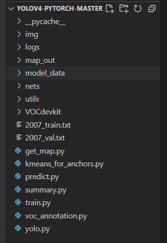
首先前往Github下载对应的仓库，下载完后利用解压软件解压，之后用编程软件打开文件夹。
注意打开的根目录必须正确，否则相对目录不正确的情况下，代码将无法运行。
一定要注意打开后的根目录是文件存放的目录。

一、数据集的准备

本文使用VOC格式进行训练，训练前需要自己制作好数据集，如果没有自己的数据集，可以通过Github连接下载VOC12+07的数据集尝试下。
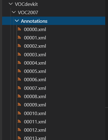
训练前将标签文件放在VOCdevkit文件夹下的VOC2007文件夹下的Annotation中。

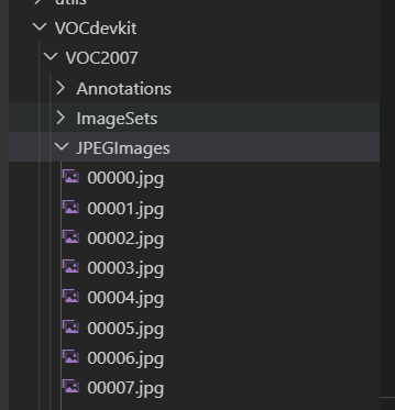
训练前将图片文件放在VOCdevkit文件夹下的VOC2007文件夹下的JPEGImages中。

此时数据集的摆放已经结束。

二、数据集的处理

在完成数据集的摆放之后，我们需要对数据集进行下一步的处理，目的是获得训练用的2007_train.txt以及2007_val.txt，需要用到根目录下的voc_annotation.py。

voc_annotation.py里面有一些参数需要设置。
分别是annotation_mode、classes_path、trainval_percent、train_percent、VOCdevkit_path，第一次训练可以仅修改classes_path

''' annotation_mode用于指定该文件运行时计算的内容 annotation_mode为0代表整个标签处理过程，包括获得VOCdevkit/VOC2007/ImageSets里面的txt以及训练用的2007_train.txt、2007_val.txt annotation_mode为1代表获得VOCdevkit/VOC2007/ImageSets里面的txt annotation_mode为2代表获得训练用的2007_train.txt、2007_val.txt '''
annotation_mode     = 0
''' 必须要修改，用于生成2007_train.txt、2007_val.txt的目标信息 与训练和预测所用的classes_path一致即可 如果生成的2007_train.txt里面没有目标信息 那么就是因为classes没有设定正确 仅在annotation_mode为0和2的时候有效 '''
classes_path        = 'model_data/voc_classes.txt'
''' trainval_percent用于指定(训练集+验证集)与测试集的比例，默认情况下 (训练集+验证集):测试集 = 9:1 train_percent用于指定(训练集+验证集)中训练集与验证集的比例，默认情况下 训练集:验证集 = 9:1 仅在annotation_mode为0和1的时候有效 '''
trainval_percent    = 0.9
train_percent       = 0.9
''' 指向VOC数据集所在的文件夹 默认指向根目录下的VOC数据集 '''
VOCdevkit_path  = 'VOCdevkit'

classes_path用于指向检测类别所对应的txt，以voc数据集为例，我们用的txt为：

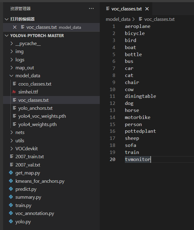
训练自己的数据集时，可以自己建立一个cls_classes.txt，里面写自己所需要区分的类别。

三、开始网络训练

通过voc_annotation.py我们已经生成了2007_train.txt以及2007_val.txt，此时我们可以开始训练了。
训练的参数较多，大家可以在下载库后仔细看注释，其中最重要的部分依然是train.py里的classes_path。

classes_path用于指向检测类别所对应的txt，这个txt和voc_annotation.py里面的txt一样！训练自己的数据集必须要修改！

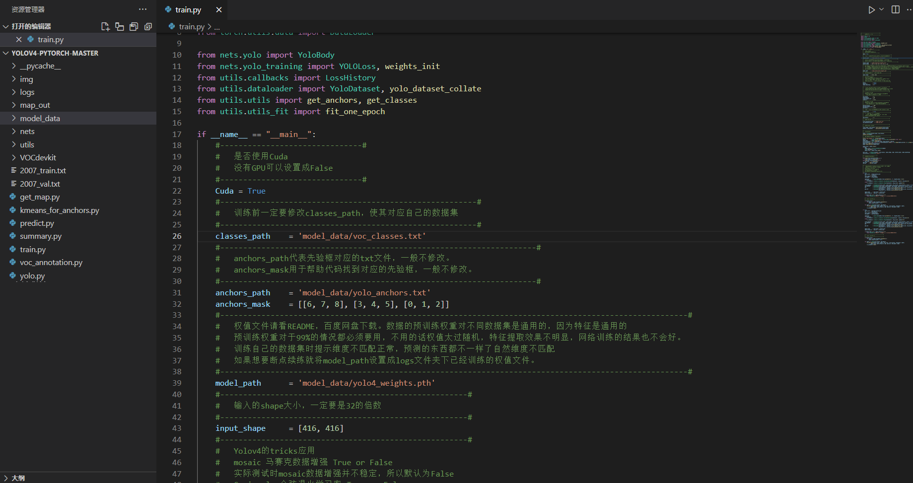
修改完classes_path后就可以运行train.py开始训练了，在训练多个epoch后，权值会生成在logs文件夹中。
其它参数的作用如下：

#--------------------------------------------------------#
# 训练前一定要修改classes_path，使其对应自己的数据集
#--------------------------------------------------------#
classes_path    = 'model_data/voc_classes.txt'
#---------------------------------------------------------------------#
# anchors_path代表先验框对应的txt文件，一般不修改。
# anchors_mask用于帮助代码找到对应的先验框，一般不修改。
#---------------------------------------------------------------------#
anchors_path    = 'model_data/yolo_anchors.txt'
anchors_mask    = [[6, 7, 8], [3, 4, 5], [0, 1, 2]]
#-------------------------------------------------------------------------------------#
# 权值文件请看README，百度网盘下载
# 训练自己的数据集时提示维度不匹配正常，预测的东西都不一样了自然维度不匹配
# 预训练权重对于99%的情况都必须要用，不用的话权值太过随机，特征提取效果不明显
# 网络训练的结果也不会好，数据的预训练权重对不同数据集是通用的，因为特征是通用的
#------------------------------------------------------------------------------------#
model_path      = 'model_data/yolo4_weight.h5'
#------------------------------------------------------#
# 输入的shape大小，一定要是32的倍数
#------------------------------------------------------#
input_shape     = [416, 416]
#------------------------------------------------------#
# Yolov4的tricks应用
# mosaic 马赛克数据增强 True or False 
# 实际测试时mosaic数据增强并不稳定，所以默认为False
# Cosine_scheduler 余弦退火学习率 True or False
# label_smoothing 标签平滑 0.01以下一般 如0.01、0.005
#------------------------------------------------------#
mosaic              = False
Cosine_scheduler    = False
label_smoothing     = 0
#----------------------------------------------------#
# 训练分为两个阶段，分别是冻结阶段和解冻阶段
# 冻结阶段训练参数
# 此时模型的主干被冻结了，特征提取网络不发生改变
# 占用的显存较小，仅对网络进行微调
#----------------------------------------------------#
Init_Epoch          = 0
Freeze_Epoch        = 50
Freeze_batch_size   = 4
Freeze_lr           = 1e-3
#----------------------------------------------------#
# 解冻阶段训练参数
# 此时模型的主干不被冻结了，特征提取网络会发生改变
# 占用的显存较大，网络所有的参数都会发生改变
# batch不能为1
#----------------------------------------------------#
UnFreeze_Epoch      = 100
Unfreeze_batch_size = 4
Unfreeze_lr         = 1e-4
#------------------------------------------------------#
# 是否进行冻结训练，默认先冻结主干训练后解冻训练。
#------------------------------------------------------#
Freeze_Train        = True
#------------------------------------------------------#
# 用于设置是否使用多线程读取数据，0代表关闭多线程
# 开启后会加快数据读取速度，但是会占用更多内存
# keras里开启多线程有些时候速度反而慢了许多
# 在IO为瓶颈的时候再开启多线程，即GPU运算速度远大于读取图片的速度。
#------------------------------------------------------#
num_workers         = 0
#----------------------------------------------------#
# 获得图片路径和标签
#----------------------------------------------------#
train_annotation_path   = '2007_train.txt'
val_annotation_path     = '2007_val.txt'

四、训练结果预测

训练结果预测需要用到两个文件，分别是yolo.py和predict.py。
我们首先需要去yolo.py里面修改model_path以及classes_path，这两个参数必须要修改。

model_path指向训练好的权值文件，在logs文件夹里。
classes_path指向检测类别所对应的txt。

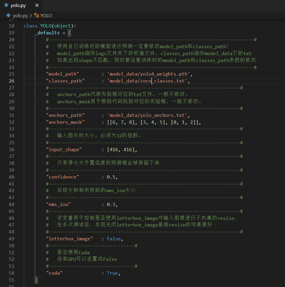
完成修改后就可以运行predict.py进行检测了。运行后输入图片路径即可检测。

发布者：全栈程序员-用户IM，转载请注明出处：https://javaforall.cn/150888.html原文链接：https://javaforall.cn

【正版授权，激活自己账号】： Jetbrains全家桶Ide使用，1年售后保障，每天仅需1毛

【官方授权正版激活】： 官方授权正版激活支持Jetbrains家族下所有IDE 使用个人JB账号...

睿智的目标检测30——Pytorch搭建YoloV4目标检测平台

睿智的目标检测30——Pytorch搭建YoloV4目标检测平台

学习前言

什么是YOLOV4

代码下载

YOLOV4改进的部分（不完全）

YOLOV4结构解析

1、主干特征提取网络Backbone

2、特征金字塔

3、YoloHead利用获得到的特征进行预测

4、预测结果的解码

5、在原图上进行绘制

YOLOV4的训练

1、YOLOV4的改进训练技巧

a)、Mosaic数据增强

b)、Label Smoothing平滑

c)、CIOU

d)、学习率余弦退火衰减

2、loss组成

a)、计算loss所需参数

b)、y_pre是什么

c)、y_true是什么。

d)、loss的计算过程

训练自己的YoloV4模型

一、数据集的准备

二、数据集的处理

三、开始网络训练

四、训练结果预测

发表回复

睿智的目标检测30——Pytorch搭建YoloV4目标检测平台

睿智的目标检测30——Pytorch搭建YoloV4目标检测平台

学习前言

什么是YOLOV4

代码下载

YOLOV4改进的部分（不完全）

YOLOV4结构解析

1、主干特征提取网络Backbone

2、特征金字塔

3、YoloHead利用获得到的特征进行预测

4、预测结果的解码

5、在原图上进行绘制

YOLOV4的训练

1、YOLOV4的改进训练技巧

a)、Mosaic数据增强

b)、Label Smoothing平滑

c)、CIOU

d)、学习率余弦退火衰减

2、loss组成

a)、计算loss所需参数

b)、y_pre是什么

c)、y_true是什么。

d)、loss的计算过程

训练自己的YoloV4模型

一、数据集的准备

二、数据集的处理

三、开始网络训练

四、训练结果预测

相关推荐

html上传图片后，在页面显示上传的图片

vue的$attrs_vue获取list集合中的对象

Java学习之注解篇

XMind快捷键汇总

网络基础知识题_无基础最易入门乐器

程序员的生存法则_程序员的一生

发表回复