大家好,又见面了,我是你们的朋友全栈君。
BN可以说是NN发展中的一个里程碑式的结构了,不增加inference时间,调参变得简单,收敛更快效果更好。
虽然提出的时间已经很久了,而且网上关于BN的解释一堆一堆的,但是博主觉得有不少解释是欠妥的,在此贴出博主贴出对caffe中BN源码的解释和自己对BN的理解,欢迎讨论。
caffe中BN的实现比较反人类。BatchNorm层单纯实现标准化,再用一个scale层添加  参数,共同完成BN。scale没啥好说的,下面开始解读BatchNorm的源码。
还是先看caffe.proto中对BN param的解释。
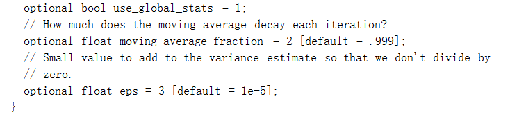
use_global_stats:为True时,使用保存的均值,方差;为False时,滑动计算均值方差。在caffe中,该参数缺省的话,TEST阶段自动置为True, 其他阶段为False. 当Finetune需要freeze BN的参数时,要把该参数置为False,否则均值,方差仍在更新;
moving_average_fraction:滑动系数,默认0.999;
eps:加在var上面的,防止标准化时分母为0。
再看hpp文件,没有什么内联函数,定义了一些blobs和前传反传函数。
#include "caffe/layer.hpp"
#include "caffe/proto/caffe.pb.h"

namespace caffe {
template <typename Dtype>
class BatchNormLayer : public Layer<Dtype> {
 public:
  explicit BatchNormLayer(const LayerParameter& param)
      : Layer<Dtype>(param) {}
  virtual void LayerSetUp(const vector<Blob<Dtype>*>& bottom,
      const vector<Blob<Dtype>*>& top);
  virtual void Reshape(const vector<Blob<Dtype>*>& bottom,
      const vector<Blob<Dtype>*>& top);

  virtual inline const char* type() const { return "BatchNorm"; }
  virtual inline int ExactNumBottomBlobs() const { return 1; } // 输入一个Blob
  virtual inline int ExactNumTopBlobs() const { return 1; } // 输出一个Blob

 protected:
  virtual void Forward_cpu(const vector<Blob<Dtype>*>& bottom,
      const vector<Blob<Dtype>*>& top);
  virtual void Forward_gpu(const vector<Blob<Dtype>*>& bottom,
      const vector<Blob<Dtype>*>& top);
  virtual void Backward_cpu(const vector<Blob<Dtype>*>& top,
      const vector<bool>& propagate_down, const vector<Blob<Dtype>*>& bottom);
  virtual void Backward_gpu(const vector<Blob<Dtype>*>& top,
     const vector<bool>& propagate_down, const vector<Blob<Dtype>*>& bottom);

  Blob<Dtype> mean_, variance_, temp_, x_norm_;
  bool use_global_stats_;
  Dtype moving_average_fraction_;
  int channels_;
  Dtype eps_;

  // extra temporarary variables is used to carry out sums/broadcasting
  // using BLAS
  Blob<Dtype> batch_sum_multiplier_;
  Blob<Dtype> num_by_chans_;
  Blob<Dtype> spatial_sum_multiplier_;
};

}  // namespace caffe

#endif  // CAFFE_BATCHNORM_LAYER_HPP_
接下来看CPP文件中的forward代码 。
#include <algorithm>
#include <vector>

#include "caffe/layers/batch_norm_layer.hpp"
#include "caffe/util/math_functions.hpp"

namespace caffe {

template <typename Dtype>
void BatchNormLayer<Dtype>::LayerSetUp(const vector<Blob<Dtype>*>& bottom,
      const vector<Blob<Dtype>*>& top) {
  BatchNormParameter param = this->layer_param_.batch_norm_param();
  moving_average_fraction_ = param.moving_average_fraction();

  // TEST阶段,use_global_stats_自动置为True。但是如果指定了该参数的话,以指定的为准
  // 所以大部分时候可以不管该参数的设置问题,只有fix BN param时需要注意
  use_global_stats_ = this->phase_ == TEST;
  if (param.has_use_global_stats())
    use_global_stats_ = param.use_global_stats();
  if (bottom[0]->num_axes() == 1)
    channels_ = 1;
  else
    channels_ = bottom[0]->shape(1);
  eps_ = param.eps();
  if (this->blobs_.size() > 0) {
    LOG(INFO) << "Skipping parameter initialization";
  } else {
    this->blobs_.resize(3);
    vector<int> sz;
    sz.push_back(channels_);
   // blobs[0]存储均值滑动和,元素个数为channel
   // blobs[1]存储方差滑动和, 元素个数为channel
   // blobs[2]存储滑动系数,元素个数为1, 三个blobs初始全部填充0
    this->blobs_[0].reset(new Blob<Dtype>(sz));
    this->blobs_[1].reset(new Blob<Dtype>(sz));
    sz[0] = 1;
    this->blobs_[2].reset(new Blob<Dtype>(sz));
    for (int i = 0; i < 3; ++i) {
      caffe_set(this->blobs_[i]->count(), Dtype(0),
                this->blobs_[i]->mutable_cpu_data());
    }
  }
  // Mask statistics from optimization by setting local learning rates
  // for mean, variance, and the bias correction to zero.
  for (int i = 0; i < this->blobs_.size(); ++i) {
    if (this->layer_param_.param_size() == i) {
      ParamSpec* fixed_param_spec = this->layer_param_.add_param();
      fixed_param_spec->set_lr_mult(0.f);
    } else {
      CHECK_EQ(this->layer_param_.param(i).lr_mult(), 0.f)
          << "Cannot configure batch normalization statistics as layer "
          << "parameters.";
    }
  }
}

template <typename Dtype>
void BatchNormLayer<Dtype>::Reshape(const vector<Blob<Dtype>*>& bottom,
      const vector<Blob<Dtype>*>& top) {
  if (bottom[0]->num_axes() >= 1)
    CHECK_EQ(bottom[0]->shape(1), channels_);
  top[0]->ReshapeLike(*bottom[0]);

  vector<int> sz;
  sz.push_back(channels_);
  mean_.Reshape(sz);
  variance_.Reshape(sz);
  temp_.ReshapeLike(*bottom[0]);
  x_norm_.ReshapeLike(*bottom[0]);
  sz[0] = bottom[0]->shape(0); // batch
  batch_sum_multiplier_.Reshape(sz);

  // spatial_sum_multiplier_元素个数为h * w,全部用1填充, 理解为一个向量
  int spatial_dim = bottom[0]->count()/(channels_*bottom[0]->shape(0));
  if (spatial_sum_multiplier_.num_axes() == 0 ||
      spatial_sum_multiplier_.shape(0) != spatial_dim) {
    sz[0] = spatial_dim;
    spatial_sum_multiplier_.Reshape(sz);
    Dtype* multiplier_data = spatial_sum_multiplier_.mutable_cpu_data();
    caffe_set(spatial_sum_multiplier_.count(), Dtype(1), multiplier_data);
  }

  // num_by_chans_元素个数为batch * channel
  // batch_sum_multiplier_元素个数为batch, 全部用1填充, 理解为一个向量
  int numbychans = channels_*bottom[0]->shape(0);
  if (num_by_chans_.num_axes() == 0 ||
      num_by_chans_.shape(0) != numbychans) {
    sz[0] = numbychans;
    num_by_chans_.Reshape(sz);
    caffe_set(batch_sum_multiplier_.count(), Dtype(1),
        batch_sum_multiplier_.mutable_cpu_data());
  }
}

template <typename Dtype>
void BatchNormLayer<Dtype>::Forward_cpu(const vector<Blob<Dtype>*>& bottom,
    const vector<Blob<Dtype>*>& top) {
  const Dtype* bottom_data = bottom[0]->cpu_data();
  Dtype* top_data = top[0]->mutable_cpu_data();
  int num = bottom[0]->shape(0); // batch
  int spatial_dim = bottom[0]->count()/(bottom[0]->shape(0)*channels_); // h * w

  // 非in-place时,复制bottom到top.
  if (bottom[0] != top[0]) {
    caffe_copy(bottom[0]->count(), bottom_data, top_data);
  }

  if (use_global_stats_) {
    // 测试阶段
    // scale = 1/blobs[2],mean_ = blobs[0]/scale,var_ = blobs[1]/scale
    // blobs[2]理论上约等于迭代的次数,实际上caffe中常常为一个999.几的定值
    // use the stored mean/variance estimates.
    const Dtype scale_factor = this->blobs_[2]->cpu_data()[0] == 0 ?
        0 : 1 / this->blobs_[2]->cpu_data()[0];
    caffe_cpu_scale(variance_.count(), scale_factor,
        this->blobs_[0]->cpu_data(), mean_.mutable_cpu_data());
    caffe_cpu_scale(variance_.count(), scale_factor,
        this->blobs_[1]->cpu_data(), variance_.mutable_cpu_data());
  } else {
	// 训练阶段
    // compute mean
	// num_by_chans_是一个batch * channel维列向量乘以1/(batch*h*w)系数,列向量每一个值是一张h*w的特征图的像素点之和
    caffe_cpu_gemv<Dtype>(CblasNoTrans, channels_ * num, spatial_dim,
        1. / (num * spatial_dim), bottom_data,
        spatial_sum_multiplier_.cpu_data(), 0.,
        num_by_chans_.mutable_cpu_data());
	// mean_ 是一个channel维列向量,每个值是batch个h*w的特征图像素点和的均值
    caffe_cpu_gemv<Dtype>(CblasTrans, num, channels_, 1.,
        num_by_chans_.cpu_data(), batch_sum_multiplier_.cpu_data(), 0.,
        mean_.mutable_cpu_data());

	// 上面第一个函数对h*w求和,第二个函数对batch维度求和,共同完成沿着batch,h,w维度求和。
  }


  // 接下来两个函数,不管是训练还是测试均需要计算
  // top = top - mean
  // subtract mean
  caffe_cpu_gemm<Dtype>(CblasNoTrans, CblasNoTrans, num, channels_, 1, 1,
      batch_sum_multiplier_.cpu_data(), mean_.cpu_data(), 0.,
      num_by_chans_.mutable_cpu_data());
  caffe_cpu_gemm<Dtype>(CblasNoTrans, CblasNoTrans, channels_ * num,
      spatial_dim, 1, -1, num_by_chans_.cpu_data(),
      spatial_sum_multiplier_.cpu_data(), 1., top_data);


  if (!use_global_stats_) {
	//训练阶段
    // compute variance using var(X) = E((X-EX)^2)
    caffe_powx(top[0]->count(), top_data, Dtype(2),
        temp_.mutable_cpu_data());  // temp_ = (X-mean)^2
	// 下面两个函数和求mean的两个函数只有输入一样,一个是bottom,一个是temp
	// variance_ = mean(temp_)
    caffe_cpu_gemv<Dtype>(CblasNoTrans, channels_ * num, spatial_dim,
        1. / (num * spatial_dim), temp_.cpu_data(),
        spatial_sum_multiplier_.cpu_data(), 0.,
        num_by_chans_.mutable_cpu_data());
    caffe_cpu_gemv<Dtype>(CblasTrans, num, channels_, 1.,
        num_by_chans_.cpu_data(), batch_sum_multiplier_.cpu_data(), 0.,
        variance_.mutable_cpu_data());  // E((X_EX)^2)

    // compute and save moving average
	// scale = 0.999*scale + 1
    this->blobs_[2]->mutable_cpu_data()[0] *= moving_average_fraction_;
    this->blobs_[2]->mutable_cpu_data()[0] += 1;
	// blobs[0]存储均值滑动和
	// blobs[0] = mean + 0.999 * blobs[0]
    caffe_cpu_axpby(mean_.count(), Dtype(1), mean_.cpu_data(),
        moving_average_fraction_, this->blobs_[0]->mutable_cpu_data());
	// 方差系数bias_correction_factor是m/(m-1)
	// blobs[1] = bias_correction_factor * var + 0.999 * blobs[1]
    int m = bottom[0]->count()/channels_;
    Dtype bias_correction_factor = m > 1 ? Dtype(m)/(m-1) : 1;
    caffe_cpu_axpby(variance_.count(), bias_correction_factor,
        variance_.cpu_data(), moving_average_fraction_,
        this->blobs_[1]->mutable_cpu_data());
  }

  // normalize variance
  // 训练测试阶段均有
  // 给var加上eps再开方,作为标准化的分母
  caffe_add_scalar(variance_.count(), eps_, variance_.mutable_cpu_data());
  caffe_powx(variance_.count(), variance_.cpu_data(), Dtype(0.5),
             variance_.mutable_cpu_data());

  // replicate variance to input size
  // 接下来两个函数是把处理后的var调整为(channels_ * num)*(spatial_dim)格式。方便对应元素相除做标准化
  caffe_cpu_gemm<Dtype>(CblasNoTrans, CblasNoTrans, num, channels_, 1, 1,
      batch_sum_multiplier_.cpu_data(), variance_.cpu_data(), 0.,
      num_by_chans_.mutable_cpu_data());
  caffe_cpu_gemm<Dtype>(CblasNoTrans, CblasNoTrans, channels_ * num,
      spatial_dim, 1, 1., num_by_chans_.cpu_data(),
      spatial_sum_multiplier_.cpu_data(), 0., temp_.mutable_cpu_data());

  // x_norm = (x-mean)/sqrt(var+eps)
  caffe_div(temp_.count(), top_data, temp_.cpu_data(), top_data);
  // TODO(cdoersch): The caching is only needed because later in-place layers
  //                 might clobber the data.  Can we skip this if they won't?
  caffe_copy(x_norm_.count(), top_data,
      x_norm_.mutable_cpu_data());
}
对于Forward函数,注释的比较详细。总结起来主要有以下几步:
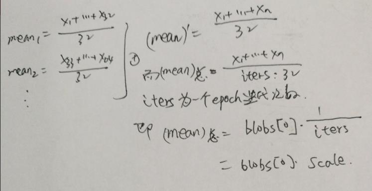
1. use_global_stats_为真时,直接用存储值计算mean和var.对应于代码中的公式。解释如下图。以batch_size = 32 ,测试时相当于使用整个train过程的所有图片作为输入,计算出mean和var。当然此处为了简单,未考虑0.999因子,直接当1使用。use_global_stats_为假时,通过两个gemv计算出mean,对应forward中第二个if;图片中关于iters解释错了,是迭代次数,在此说明一下
2. top = top – mean,不管训练还是测试都做这一步;
3. 只有use_global_stats_为假时有这一步。先计算出var,然后更新滑动系数和,均值滑动和 和 方差滑动和。此处要注意的是样本的是总体均值的无偏估计,所以存储均值时,直接累加;但是样本的方差不是总体的无偏估计,总体方差均值是样本方差均值的,所以存储方差为以后估计总体方差时,前乘了这样一个系数再累加;
4.至此,不管use_global_stats_为啥值,mean,var均已得知,此步骤换算得到标准化的结果。
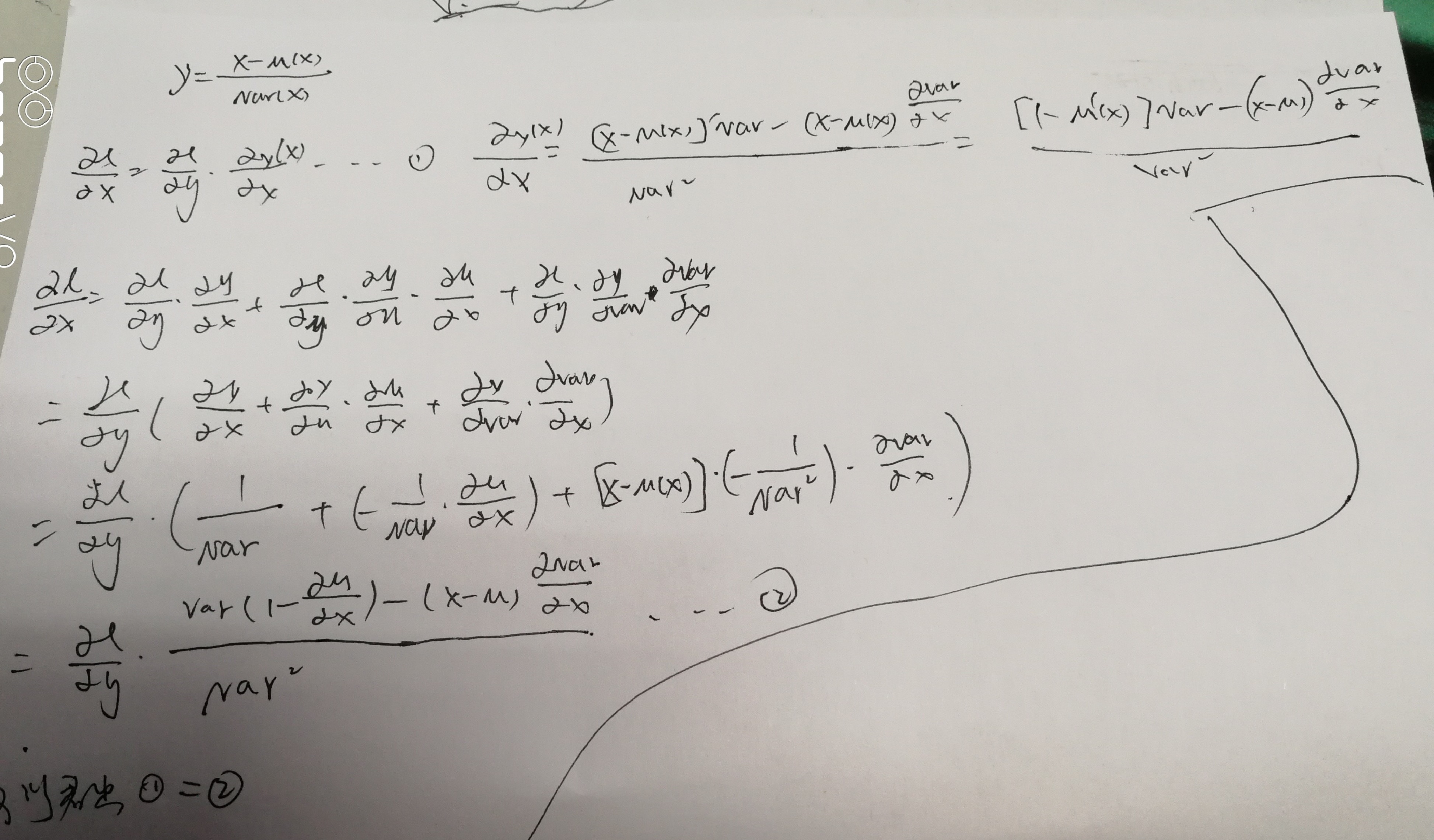
对于Backward,先推导一组公式。可以看出,将mean和var看成x的函数直接用y对x求导,和将mean,var看成中间变量,分别利用y对x的导数,mean对x的导数和var对x的导数之和,求出来的结果是一样的。caffe中的实现用的是后者的方法。
再贴上backward的cpp代码。
template <typename Dtype>
void BatchNormLayer<Dtype>::Backward_cpu(const vector<Blob<Dtype>*>& top,
const vector<bool>& propagate_down,
const vector<Blob<Dtype>*>& bottom) {
const Dtype* top_diff;
if (bottom[0] != top[0]) {
top_diff = top[0]->cpu_diff();
} else {
caffe_copy(x_norm_.count(), top[0]->cpu_diff(), x_norm_.mutable_cpu_diff());
top_diff = x_norm_.cpu_diff();
}
Dtype* bottom_diff = bottom[0]->mutable_cpu_diff();
if (use_global_stats_) {
// use_global_stats_为真时,采用储存的数据计算均值,方差。
// 不仅用于测试,也有可能用于train的时候fix参数
// 反传的时候将顶层传来的梯度乘以sqrt(var+eps)即可。因为此时该层相当于scale层
caffe_div(temp_.count(), top_diff, temp_.cpu_data(), bottom_diff);
return;
}
const Dtype* top_data = x_norm_.cpu_data();
int num = bottom[0]->shape()[0];
int spatial_dim = bottom[0]->count()/(bottom[0]->shape(0)*channels_);
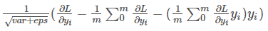
// if Y = (X-mean(X))/(sqrt(var(X)+eps)), then
//
// dE(Y)/dX =
// (dE/dY - mean(dE/dY) - mean(dE/dY \cdot Y) \cdot Y)
// ./ sqrt(var(X) + eps)
//
// where \cdot and ./ are hadamard product and elementwise division,
// respectively, dE/dY is the top diff, and mean/var/sum are all computed
// along all dimensions except the channels dimension. In the above
// equation, the operations allow for expansion (i.e. broadcast) along all
// dimensions except the channels dimension where required.
// sum(dE/dY \cdot Y)
caffe_mul(temp_.count(), top_data, top_diff, bottom_diff);
caffe_cpu_gemv<Dtype>(CblasNoTrans, channels_ * num, spatial_dim, 1.,
bottom_diff, spatial_sum_multiplier_.cpu_data(), 0.,
num_by_chans_.mutable_cpu_data());
caffe_cpu_gemv<Dtype>(CblasTrans, num, channels_, 1.,
num_by_chans_.cpu_data(), batch_sum_multiplier_.cpu_data(), 0.,
mean_.mutable_cpu_data());
// reshape (broadcast) the above
caffe_cpu_gemm<Dtype>(CblasNoTrans, CblasNoTrans, num, channels_, 1, 1,
batch_sum_multiplier_.cpu_data(), mean_.cpu_data(), 0.,
num_by_chans_.mutable_cpu_data());
caffe_cpu_gemm<Dtype>(CblasNoTrans, CblasNoTrans, channels_ * num,
spatial_dim, 1, 1., num_by_chans_.cpu_data(),
spatial_sum_multiplier_.cpu_data(), 0., bottom_diff);
// sum(dE/dY \cdot Y) \cdot Y
caffe_mul(temp_.count(), top_data, bottom_diff, bottom_diff);
// sum(dE/dY)-sum(dE/dY \cdot Y) \cdot Y
caffe_cpu_gemv<Dtype>(CblasNoTrans, channels_ * num, spatial_dim, 1.,
top_diff, spatial_sum_multiplier_.cpu_data(), 0.,
num_by_chans_.mutable_cpu_data());
caffe_cpu_gemv<Dtype>(CblasTrans, num, channels_, 1.,
num_by_chans_.cpu_data(), batch_sum_multiplier_.cpu_data(), 0.,
mean_.mutable_cpu_data());
// reshape (broadcast) the above to make
// sum(dE/dY)-sum(dE/dY \cdot Y) \cdot Y
caffe_cpu_gemm<Dtype>(CblasNoTrans, CblasNoTrans, num, channels_, 1, 1,
batch_sum_multiplier_.cpu_data(), mean_.cpu_data(), 0.,
num_by_chans_.mutable_cpu_data());
caffe_cpu_gemm<Dtype>(CblasNoTrans, CblasNoTrans, num * channels_,
spatial_dim, 1, 1., num_by_chans_.cpu_data(),
spatial_sum_multiplier_.cpu_data(), 1., bottom_diff);
// dE/dY - mean(dE/dY)-mean(dE/dY \cdot Y) \cdot Y
caffe_cpu_axpby(temp_.count(), Dtype(1), top_diff,
Dtype(-1. / (num * spatial_dim)), bottom_diff);
// note: temp_ still contains sqrt(var(X)+eps), computed during the forward
// pass.
caffe_div(temp_.count(), bottom_diff, temp_.cpu_data(), bottom_diff);
}backward没啥好说的,完全按照公式来的,唯一要注意的就是 use_global_stats_为真时,该层相当于scale层,将传来的梯度乘以sqrt(var+eps)即可。
反向传播公式如下图:
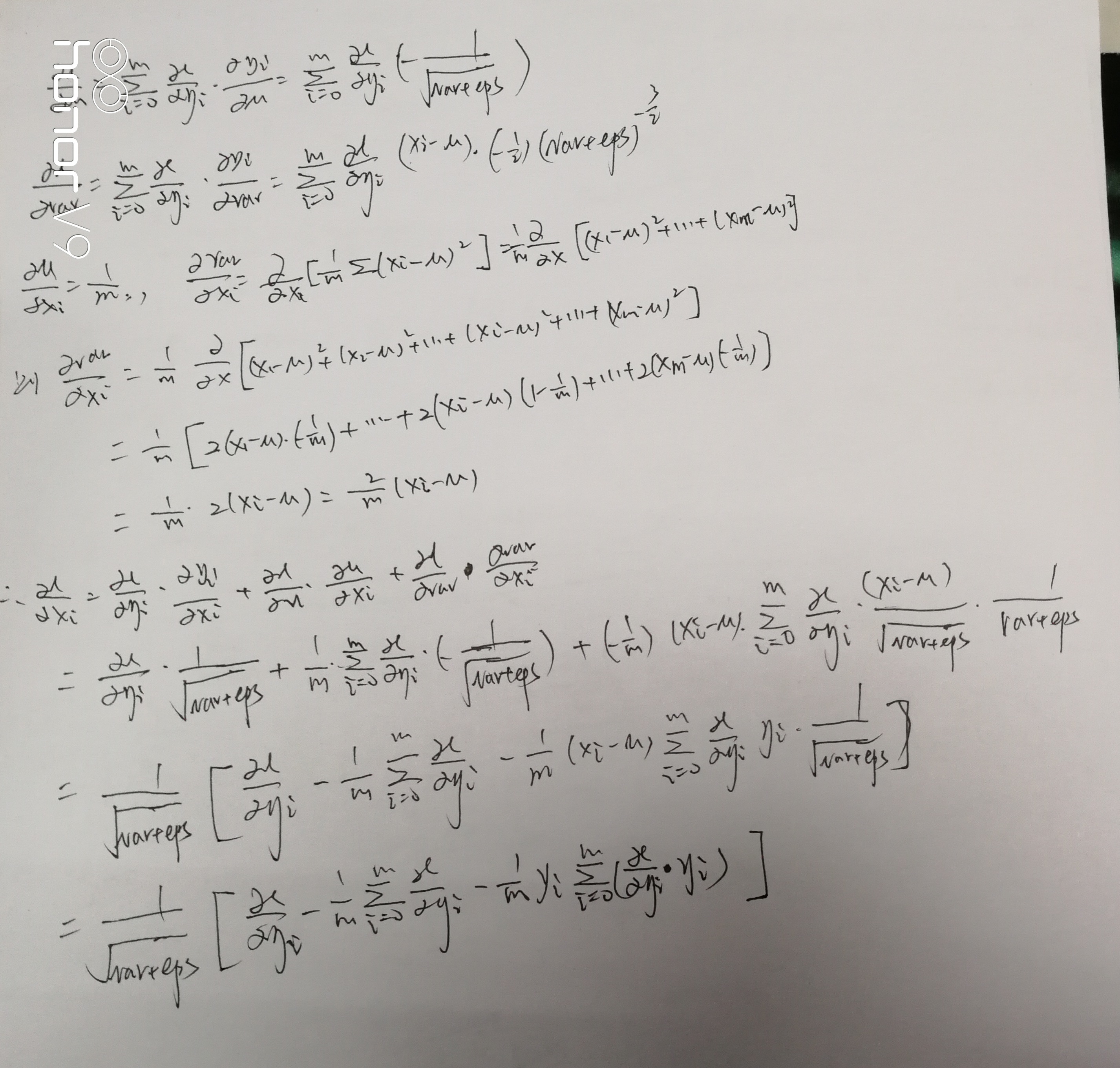
总的来看就是下图的公式,代码首先求最后一部分,然后求中间的部分,最后得出结果。
关于BN的实现细节就说到这儿,以后想到再说,下面博主分析为什么BN可以work
华丽的分割线
博主坚信万物都能从公式中看到规律,哈哈哈哈。
将BN放在模型中,如下图所示。和是BN 训练的scale参数。考虑BN为什么可以work.
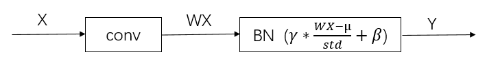
1. 当W伸缩变换时,即时
发布者:全栈程序员-用户IM,转载请注明出处:https://javaforall.cn/143067.html原文链接:https://javaforall.cn
【正版授权,激活自己账号】: Jetbrains全家桶Ide使用,1年售后保障,每天仅需1毛
【官方授权 正版激活】: 官方授权 正版激活 支持Jetbrains家族下所有IDE 使用个人JB账号...
