大家好,又见面了,我是你们的朋友全栈君。
因为需要用到和机器人相关的东西,就用到了这个工具箱,作者官网 http://www.petercorke.com/Robotics_Toolbox.html
我上传到CSDN,有需要的同学可以自行下载。robot-9.8_2013_2_12.zip_机械臂DH法建模-数据集文档类资源-CSDN文库
老爷子很厉害,那本《Robotics, Vision & Control》就是他本人写的,可以看做是工具箱的一个详细说明书。另外,在网站那里提到了rvctools/robot/robot.pdf这个pdf可以看做一个函数的使用说明文档,有不懂的函数可以在pdf中查查它的API。
关于安装方法可以参考http://blog.sina.com.cn/s/blog_a16714bf0101hycq.html
将Matlab_Robotic_Toolbox_v9.8.rar解压后,放在matlab的安装目录下,最好是放在toolbox文件夹里,利用matlab的工具栏的setpath,将文件夹Matlab_Robotic_Toolbox_v9.8\rvctools设置为matlab的搜索目录,在command window输入“startup_rvc”运行startup_rvc.m文件,自动配置工具箱的环境变量。
- 将Matlab_Robotic_Toolbox_v9.8.rar解压到C:\Program Files\MATLAB\R2017b\toolbox
- >> addpath(genpath(‘C:\Program Files\MATLAB\R2017b\toolbox\rvctools’))
- >> savepath
========2019========
第二种安装方法就是下载后缀名为mltbx的工具箱文件,双击就可以安装了。
卸载:
- 进入 MATLAB 主界面,点击 HOME > Add-Ons > Manage Add-Ons,弹出窗口:Add-On Manager
- 找到工具箱 Robotic Toolbox,然后点击右侧的 Uninstall,即可完成卸载。
========2019========
最后,你可以在command window输入“ver”,查看机器人工具箱是否已经安装成功了。command window会列出所有的工具箱,其中Robotics Toolbox已经包含在里面。
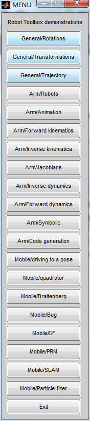
首先,输入rtbdemo可以看到一个列表,这个列表包含了常用的一些功能。我们也可以通过学习这个来快速上手这个工具箱。

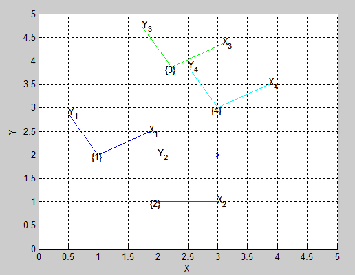
- 旋转
%二维平面内的姿态(x, y, theta), Special Euclidean(2)
clear;
clc;
T1 = se2(1, 2, 30*pi/180)
trplot2(T1, 'frame', '1', 'color', 'b')
T2 = se2(2, 1, 0)
hold on
trplot2(T2, 'frame', '2', 'color', 'r');
T3 = T1*T2
trplot2(T3, 'frame', '3', 'color', 'g');
T4 = T2*T1
trplot2(T4, 'frame', '4', 'color', 'c');
P = [3 ; 2 ];
plot_point(P, '*');% 画出点的方位(world)
P1 = inv(T1) * [P; 1] % 点P在坐标系{1}中的方位,P齐次,原始式 h2e(inv(T1) * e2h(P))
axis([0 5 0 5]);

P2 = homtrans( inv(T2), P) % 点P在坐标系{2}中的方位
注意:点为列向量
>> R = rotx(pi/2)
R =
1.0000 0 0
0 0.0000 -1.0000
0 1.0000 0.0000
>> tranimate(R) 动画显示
>> det(R) 行列式
>> R = rotx(30, ‘deg’) * roty(50, ‘deg’) * rotz(10, ‘deg’)
>> trplot(R) 最终形态
>>[theta,vec] = tr2angvec(R) 绕空间中的轴vec旋转theta角
>> eul = tr2eul(R) 转化为Eular角(Z,Y,Z)
>> rpy = tr2rpy(R) 转化为RPY(X,Y,Z),相对于上一个坐标系
H=eul2tr(-2.89091, 2.87881, 1.06893); tr2rpy(H,’zyx’)
>> q = Quaternion(R)
Quaternion(eul2tr(0.871757,2.94109,-1.64967)) Z, Y, Z
>> q.R
>>q1 = Quaternion( rotx(pi/2) )
>>q2 = Quaternion( roty(pi/2) )
>> q1 * q2
=======================三维坐标==============================
x_nominal_b = 0.34;
 y_nominal_b = 0.19;
 z_nominal_b = -0.42;

 LF=[x_nominal_b   y_nominal_b z_nominal_b];
 RF=[  x_nominal_b  -y_nominal_b z_nominal_b];
 LH= [-x_nominal_b   y_nominal_b z_nominal_b];
 RH=[ -x_nominal_b  -y_nominal_b z_nominal_b];

 T=[LF ;RF ;LH ;RH];

 a=T(:,1);
 b=T(:,2);
 c=T(:,3);
%  scatter3( a,b,c,'b')
 plot3(a,b,c,'b.','MarkerSize',5)
 grid on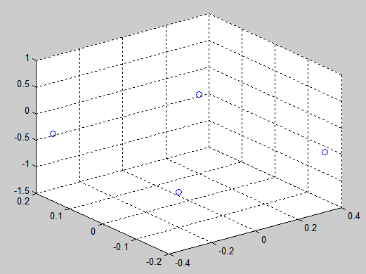
clc;
clear;
close all;
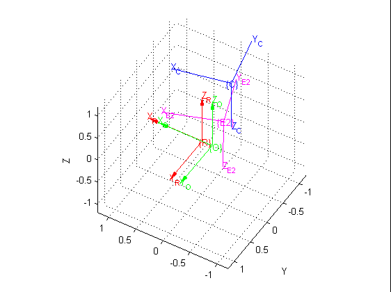
t1 = eye(4);
trplot(t1,'frame','R','arrow','width', '1', 'color', 'r', 'text_opts', {'FontSize', 10, 'FontWeight', 'light'},'view', [-0.3 0.5 0.6],'thick',0.9,'dispar',0.8 );
hold on;
robotHcam =[ -120.2117270943047, -700.033498810312, 759.864364912089, -3.137243821744305, -0.007451761425653, -0.207643158709979 ];
robotHcam(1,1) = robotHcam(1,1) /1000.0;
robotHcam(1,2) = robotHcam(1,2) /1000.0;
robotHcam(1,3) = robotHcam(1,3) /1000.0;
robotHcam1 = transl(robotHcam(1,1), robotHcam(1,2), robotHcam(1,3)) * trotx(robotHcam(1,4)) * troty(robotHcam(1,5))* trotz(robotHcam(1,6))
trplot(robotHcam1,'frame','C');
eef_real = [-0.0190283,-0.63227,-0.101349,-3.09773,-0.0104572,-0.33805];% -179.545 15.2654 -4.47882
robotHobj_real = transl(eef_real(1,1), eef_real(1,2), eef_real(1,3)) * trotx(eef_real(1,4)) * troty(eef_real(1,5))* trotz(eef_real(1,6))
trplot(robotHobj_real,'frame','E2', 'color', 'magenta')%cyan
camHobj = [ 0.082430 -0.075731 0.858318 -3.124834 -3.139422 3.051156];
camHobj1 = transl(camHobj(1,1), robotHcam(1,2), robotHcam(1,3)) * trotx(robotHcam(1,4)) * troty(robotHcam(1,5))* trotz(robotHcam(1,6));
robotHobj = robotHcam1 * camHobj1
trplot(robotHobj,'frame','O','arrow','width', '1', 'color', 'g');
============ Matlab 2018b和机器人工具箱 ===================
baseHyake  =[ -0.085 -0.509 0.205 0.934 -0.138 0.073 -0.322];
trvec = baseHyake(:, 1:3)
qua = quaternion(baseHyake(1,7), baseHyake(1,4), baseHyake(1,5), baseHyake(1,6))

baseHyake_homo = trvec2tform(trvec) * quat2tform(qua)

% rtb工具箱
trplot(baseHyake_homo, 'frame', 'yake', 'width', '1', 'color', 'black');

hold on;
% startup_rvc
World = eye(4)


trplot(World,'frame', 'W', 'width', '1', 'color', 'r');
2. 平移
>> transl(0.5, 0.0, 0.0)
ans =
1.0000 0 0 0.5000
0 1.0000 0 0
0 0 1.0000 0
0 0 0 1.0000
>> troty(pi/2) 绕y轴旋转pi/2
ans =
0.0000 0 1.0000 0
0 1.0000 0 0
-1.0000 0 0.0000 0
0 0 0 1.0000
>> t = transl(0.5, 0.0, 0.0) * troty(pi/2) * trotz(-pi/2)
% If thistransformation represented the origin of a new coordinate frame with respect
% to the worldframe origin (0, 0, 0), that new origin would be given by
>> t * [0 0 0 1]’
ans =
0.5000
0
0
1.0000
3. 轨迹
3.1 五次多项式轨迹规划
通常的轨迹规划限制条件:起始终止速度、加速度为0,设定起点和终点,一共6个条件,所以最容易想到的是5次多项式轨迹规划。
clear;
clc;
p0 = -1;% 定义初始点及终点位置
p1 = 2;
p = tpoly(p0, p1, 50);% 取步长为50
figure(1);

%%
plot(p);%绘图,可以看到在初始点及终点的一、二阶导均为零
[p,pd,pdd] = tpoly(p0, p1, 50);%得到位置、速度、加速度 tpoly为五阶多项式(这里的50步长并非限制条件)
figure(2);

subplot(3,1,1); plot(p); xlabel('Time'); ylabel('p');
title('初始和终止速度都为0');
grid on;
subplot(3,1,2); plot(pd); xlabel('Time'); ylabel('pd');
grid on;
subplot(3,1,3); plot(pdd); xlabel('Time'); ylabel('pdd');
grid on;

%%
[s,sd,sdd] = tpoly(0, 1, 50, 0.5, 0); % 初始速度0.5,终点速度0

figure(3);
subplot(3,1,1); plot(s); xlabel('Time'); ylabel('s');
title('初始和终止速度为0.5和0')
hold on;
n = find(s == max(s));
plot(n, s(n),'o');
cell_string{1} = ['smax = ' num2str(s(n))]; % 多行文本
cell_string{2} = ['time = ' num2str(n)];

 text(n, s(n) -3, cell_string);
 hold off;
grid on;
subplot(3,1,2); plot(sd); xlabel('Time'); ylabel('sd');
grid on;
subplot(3,1,3); plot(sdd); xlabel('Time'); ylabel('sdd');
grid on;
下图为路径曲线,速度曲线和加速度曲线。
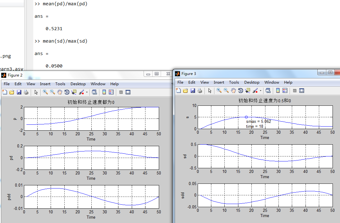
可以从图中看出初始和终止速度都为0时(左图),平均速度只有52%达到了峰值,也就是说机器人运行效率不高。而当初始和终止速度分别为0.5和0时(右图),除了平均速度的问题外,它的轨迹漂移比较大,从位置0到1的运动,最大达到了5.062。因此就引入了抛物线轨迹规划。
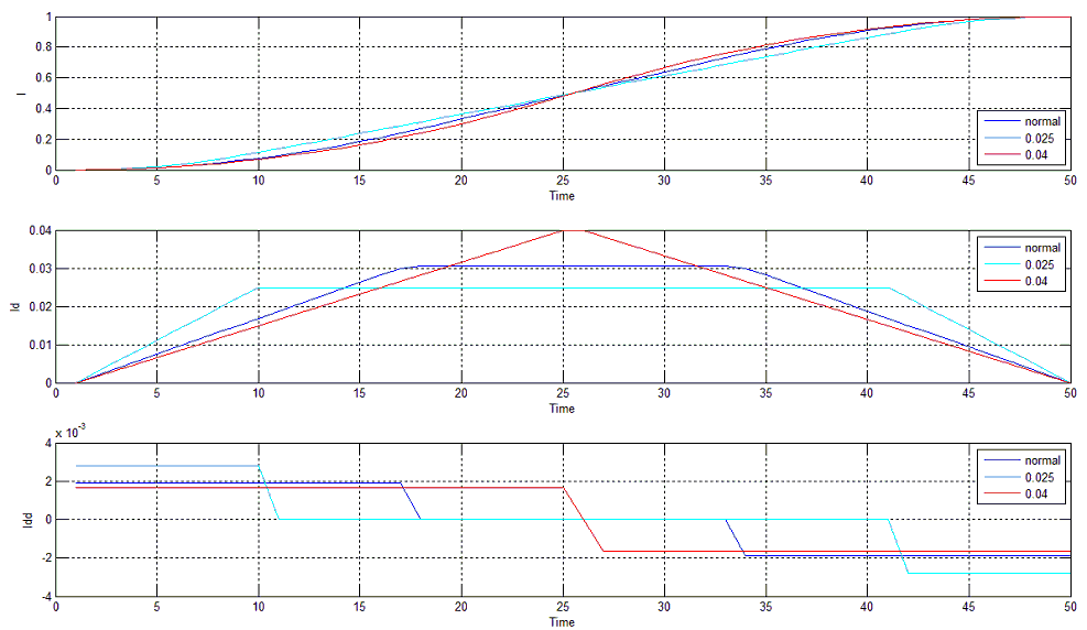
3.2 抛物线轨迹规划
抛物线轨迹规划就是起始段和终止段为抛物线,中间有部分为直线匀速段。限制条件为起始终止位置、起始终止速度、总时间。匀速段的速度在一定条件也可以作为限制条件。
[l,ld,ldd] = lspb(p0, p1, 50); % Linear Segment(匀速) with Parabolic(抛物线) Blends(过渡)注意这里的总步长是一个限制条件
figure(4);
subplot(3,1,1); plot(l); xlabel('Time'); ylabel('l');
grid on;
subplot(3,1,2); plot(ld); xlabel('Time'); ylabel('ld');% 可以看到速度是呈梯形
grid on;
subplot(3,1,3); plot(ldd); xlabel('Time'); ylabel('ldd');
grid on;
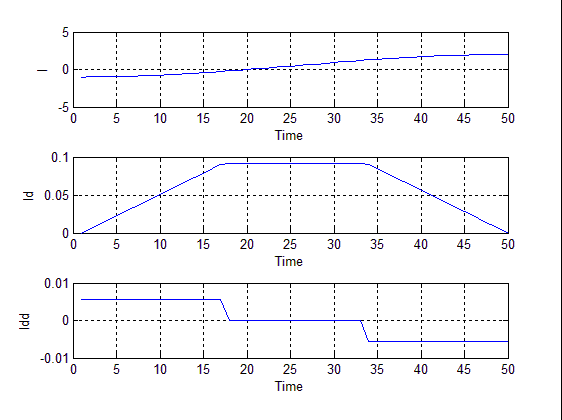
当设定匀速段的速度时,轨迹会有不同的反应。随着速度增加,他的匀速时间变短了,而且加速度会增大,也就是说震动会加大。匀速段的速度不能太大也不能太小,否则会无解。因为他是一个Over constraied system,这里有5个constrains(总时间,初始终止位置,初始终止速度)但是有6个freedom(抛物线过渡时间,抛物线方程的三个量,直线方程的两个量)。相当于有5个未知数但是有6个方程,无解。
在《机器人学导论–分析、控制及应用》——Saeed B.Niku 孙富春这本书P145提到,因为加速减速是对称的,vmax = 2(lf – l0)/ tf, lf和l0指终止和初始位置,tf是总时间。
这里vmax = 2(1-0)/ 50 = 0.04, 匀速段最大速度为0.04.不然就会没有匀速段的时间
clear;
clc;
p0 = -1;% 定义初始点及终点位置
p1 = 2;
p = tpoly(p0, p1, 50);% 取步长为50
figure(1);

%%
plot(p);%绘图,可以看到在初始点及终点的一、二阶导均为零
[p,pd,pdd] = tpoly(p0, p1, 50);%得到位置、速度、加速度
%p为五阶多项式,速度、加速度均在一定范围内
figure(2);

subplot(3,1,1); plot(p); xlabel('Time'); ylabel('p');
title('初始和终止速度都为0');
grid on;
subplot(3,1,2); plot(pd); xlabel('Time'); ylabel('pd');
grid on;
subplot(3,1,3); plot(pdd); xlabel('Time'); ylabel('pdd');
grid on;

%%
[s,sd,sdd] = tpoly(0, 1, 50, 0.5, 0); % 初始速度0.5,终点速度0

figure(3);
subplot(3,1,1); plot(s); xlabel('Time'); ylabel('s');
title('初始和终止速度为0.5和0')
hold on;
n = find(s == max(s));
plot(n, s(n),'o');
cell_string{1} = ['smax = ' num2str(s(n))]; % 多行文本
cell_string{2} = ['time = ' num2str(n)];

 text(n, s(n) -3, cell_string);
 hold off;
grid on;
subplot(3,1,2); plot(sd); xlabel('Time'); ylabel('sd');
grid on;
subplot(3,1,3); plot(sdd); xlabel('Time'); ylabel('sdd');
grid on;
%%
[l,ld,ldd] = lspb(0, 1, 50); % Linear Segment(匀速) with Parabolic(抛物线) Blends(过渡)
figure(4);

subplot(3,1,1); plot(l); xlabel('Time'); ylabel('l');
grid on;
hold on;
subplot(3,1,2); plot(ld); xlabel('Time'); ylabel('ld');% 可以看到速度是呈梯形
grid on;
hold on;
subplot(3,1,3); plot(ldd); xlabel('Time'); ylabel('ldd');
grid on;
hold on;

[l,ld,ldd] = lspb(0, 1, 50, 0.025);
subplot(3,1,1); plot(l,'c'); xlabel('Time'); ylabel('l');
grid on;

subplot(3,1,2); plot(ld, 'c'); xlabel('Time'); ylabel('ld');
grid on;

subplot(3,1,3); plot(ldd,'c'); xlabel('Time'); ylabel('ldd');
grid on;

[l,ld,ldd] = lspb(0, 1, 50, 0.04);
subplot(3,1,1); plot(l,'r'); xlabel('Time'); ylabel('l');
grid on;
hold off;
legend('normal','0.025','0.04','location','southeast');

subplot(3,1,2); plot(ld,'r'); xlabel('Time'); ylabel('ld');
grid on;
hold off;
legend('normal','0.025','0.04','location','northeast');

subplot(3,1,3); plot(ldd,'r'); xlabel('Time'); ylabel('ldd');
grid on;
hold off;
legend('normal','0.025','0.04','location','northeast');
3.3 多重分割轨迹规划
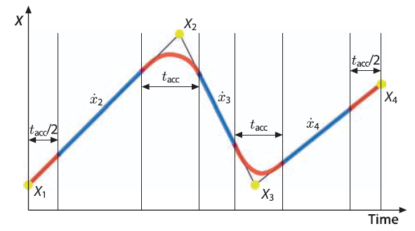
>> via = [4,1; 4,4; 5,2; 2,5];
>> q = mstraj(via, [2,1], [], [4, 1], 0.05, 0);% 每个坐标系上的最大速度,分段时间(与前面最大速度二者取一个),初始速度,样本间隔,加速时间,All axes reach their via points at the same time.
>> plot(q,'DisplayName','q')
% mstraj的位移、速度和加速度曲线P48
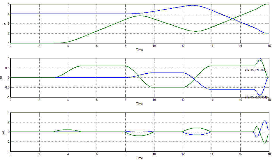
clc;
clf;
close all;
d=0.05;
% t=0:d:400;
via = [ 4,1; 4,4; 5,2; 2,5 ];
p=mstraj(via, [2,1], [], [4,1], 0.05, 2);
mstraj(via, [2,1], [], [4,1], 0.05, 2);
pd(:,1)=gradient(p(:,1))/d;
pd(:,2)=gradient(p(:,2))/d;
pdd(:,1)=gradient(pd(:,1))/d;
pdd(:,2)=gradient(pd(:,2))/d;
subplot(3,1,1);plot([t,t],p,'Linewidth',2);xlabel('Time');ylabel('p');grid on;
subplot(3,1,2);plot([t,t],pd,'Linewidth',2);xlabel('Time');ylabel('pd');grid on;
hold on;
max1=find(abs(pd(:,1))==max(abs(pd(:,1))))
max2=find(abs(pd(:,2))==max(abs(pd(:,2))))
plot(t(max1),pd(max1,1),'*');%描点画出关节1的最大速度点
plot(t(max2),pd(max2,2),'o','markersize',12);%描点画出关节2的最大速度点
text(t(max1,1)-1,pd(max1,1)-0.3,['(',num2str(t(max1,1)),',',num2str(pd(max1,1)),')']);% 标注极值点
text(t(max2,1)-1,pd(max2,1)+1.3,['(',num2str(t(max2,1)),',',num2str(pd(max2,2)),')']);
subplot(3,1,3);plot([t,t],pdd,'Linewidth',2);xlabel('Time');ylabel('pdd');grid on;
相比抛物线轨迹规划,匀速段和加速度段较好,但是他牺牲了位置点的精确性,只是趋近于途经点。
平移与旋转复合运动
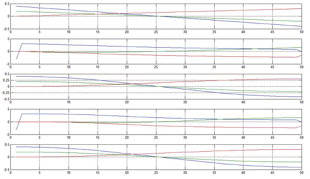
%% P49

T0 = transl(0.4, 0.2, 0) * trotx(pi);
T1 = transl(-0.4, -0.2, 0.3) * troty(pi/2) * trotz(-pi/2);
Ts = trinterp(T0, T1, [0:49]/49); % 范围是【0,1】
about(Ts);
Ts(:, :, 1)
P = transl(Ts);% 平移部分
about(P)
figure(5);
subplot(5,1,1);plot(P,'DisplayName','Translate1');grid on;

rpy = tr2rpy(Ts);% 旋转部分
subplot(5,1,2);
plot(rpy,'DisplayName','RPY1');grid on;

Ts2 = trinterp(T0, T1, lspb(0, 1, 50));% 平滑平移部分
subplot(5,1,3);plot(transl(Ts2),'DisplayName','Translate2');grid on;set(gca,'XTick',0:10:50, 'YTick',[-0.5, -0.25,  0, 0.25, 0.5]);

subplot(5,1,4);plot(tr2rpy(Ts2),'DisplayName','RPY2');grid on;

Ts3 = ctraj(T0, T1, 50);% ctraj替代trinterp(T0, T1, lspb(0, 1, 50));
subplot(5,1,5);plot(transl(Ts3),'DisplayName','Translate2');grid on;
发布者:全栈程序员-用户IM,转载请注明出处:https://javaforall.cn/132428.html原文链接:https://javaforall.cn
【正版授权,激活自己账号】: Jetbrains全家桶Ide使用,1年售后保障,每天仅需1毛
【官方授权 正版激活】: 官方授权 正版激活 支持Jetbrains家族下所有IDE 使用个人JB账号...
