lstm时间序列预测模型

时间序列-LSTM模型 (Time Series – LSTM Model)

Now, we are familiar with statistical modelling on time series, but machine learning is all the rage right now, so it is essential to be familiar with some machine learning models as well. We shall start with the most popular model in time series domain − Long Short-term Memory model.

现在，我们已经很熟悉时间序列的统计建模，但是机器学习现在非常流行，因此也必须熟悉某些机器学习模型。 我们将从时间序列域中最流行的模型开始-长短期记忆模型。

LSTM is a class of recurrent neural network. So before we can jump to LSTM, it is essential to understand neural networks and recurrent neural networks.

LSTM是一类递归神经网络。 因此，在进入LSTM之前，必须了解神经网络和递归神经网络。

神经网络 (Neural Networks)

An artificial neural network is a layered structure of connected neurons, inspired by biological neural networks. It is not one algorithm but combinations of various algorithms which allows us to do complex operations on data.

人工神经网络是受生物神经网络启发的连接神经元的分层结构。 它不是一种算法，而是多种算法的组合，使我们能够对数据进行复杂的操作。

递归神经网络 (Recurrent Neural Networks)

It is a class of neural networks tailored to deal with temporal data. The neurons of RNN have a cell state/memory, and input is processed according to this internal state, which is achieved with the help of loops with in the neural network. There are recurring module(s) of ‘tanh’ layers in RNNs that allow them to retain information. However, not for a long time, which is why we need LSTM models.

它是为处理时间数据而量身定制的一类神经网络。 RNN的神经元具有细胞状态/内存，并根据此内部状态处理输入，这是借助神经网络中的循环来实现的。 RNN中有“ tanh”层的重复模块，可让它们保留信息。 但是，不是很长一段时间，这就是为什么我们需要LSTM模型。

LSTM (LSTM)

It is special kind of recurrent neural network that is capable of learning long term dependencies in data. This is achieved because the recurring module of the model has a combination of four layers interacting with each other.

它是一种特殊的循环神经网络，能够学习数据的长期依赖性。 之所以能够实现这一目标，是因为模型的重复模块具有相互交互的四层组合。

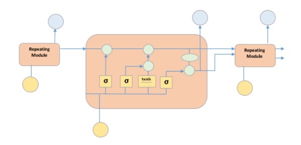
The picture above depicts four neural network layers in yellow boxes, point wise operators in green circles, input in yellow circles and cell state in blue circles. An LSTM module has a cell state and three gates which provides them with the power to selectively learn, unlearn or retain information from each of the units. The cell state in LSTM helps the information to flow through the units without being altered by allowing only a few linear interactions. Each unit has an input, output and a forget gate which can add or remove the information to the cell state. The forget gate decides which information from the previous cell state should be forgotten for which it uses a sigmoid function. The input gate controls the information flow to the current cell state using a point-wise multiplication operation of ‘sigmoid’ and ‘tanh’ respectively. Finally, the output gate decides which information should be passed on to the next hidden state

上图显示了黄色方框中的四个神经网络层，绿色圆圈中的点智能算子，黄色圆圈中的输入，蓝色圆圈中的单元状态。 LSTM模块具有单元状态和三个门，这三个门为它们提供了从每个单元中选择性地学习，取消学习或保留信息的能力。 LSTM中的单元状态仅允许一些线性交互作用，从而使信息流经这些单元而不会被更改。 每个单元都有一个输入，输出和一个忘记门，可以将信息添加或删除到单元状态。 遗忘门决定使用S形函数应忘记先前单元状态中的哪些信息。 输入门分别使用“ Sigmoid”和“ tanh”的逐点乘法运算将信息流控制为当前单元状态。 最后，输出门决定应将哪些信息传递到下一个隐藏状态

Now that we have understood the internal working of LSTM model, let us implement it. To understand the implementation of LSTM, we will start with a simple example − a straight line. Let us see, if LSTM can learn the relationship of a straight line and predict it.

现在我们已经了解了LSTM模型的内部工作原理，让我们实现它。 为了理解LSTM的实现，我们将从一个简单的示例开始-一条直线。 让我们看看，LSTM是否可以学习直线的关系并对其进行预测。

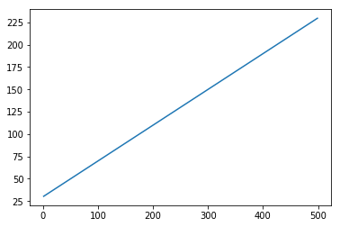
First let us create the dataset depicting a straight line.

首先，让我们创建描述直线的数据集。

In [402]:

在[402]中：

x = numpy.arange (1,500,1)
y = 0.4 * x + 30
plt.plot(x,y)

Out[402]:

出[402]：

[<matplotlib.lines.Line2D at 0x1eab9d3ee10>]

In [403]:

在[403]中：

trainx, testx = x[0:int(0.8*(len(x)))], x[int(0.8*(len(x))):]
trainy, testy = y[0:int(0.8*(len(y)))], y[int(0.8*(len(y))):]
train = numpy.array(list(zip(trainx,trainy)))
test = numpy.array(list(zip(trainx,trainy)))

Now that the data has been created and split into train and test. Let’s convert the time series data into the form of supervised learning data according to the value of look-back period, which is essentially the number of lags which are seen to predict the value at time ‘t’.

现在已经创建了数据，并将其拆分为训练和测试。 让我们根据回溯期的值将时间序列数据转换为监督学习数据的形式，回溯期的值本质上是指可以预测时间“ t”时的滞后次数。

So a time series like this −

所以这样的时间序列-

time variable_x
t1  x1
t2  x2
 :   :
 :   :
T   xT

When look-back period is 1, is converted to −

当回溯期为1时，转换为-

x1   x2
x2   x3
 :    :
 :    :
xT-1 xT

In [404]:

在[404]中：

def create_dataset(n_X, look_back):
   dataX, dataY = [], []
   for i in range(len(n_X)-look_back):
      a = n_X[i:(i+look_back), ]
      dataX.append(a)
      dataY.append(n_X[i + look_back, ])
   return numpy.array(dataX), numpy.array(dataY)

In [405]:

在[405]中：

look_back = 1
trainx,trainy = create_dataset(train, look_back)
testx,testy = create_dataset(test, look_back)

trainx = numpy.reshape(trainx, (trainx.shape[0], 1, 2))
testx = numpy.reshape(testx, (testx.shape[0], 1, 2))

Now we will train our model.

现在，我们将训练模型。

Small batches of training data are shown to network, one run of when entire training data is shown to the model in batches and error is calculated is called an epoch. The epochs are to be run ‘til the time the error is reducing.

将小批量的训练数据显示给网络，一次将整个训练数据分批显示给模型并且计算出误差时的一次运行称为时期。 直到错误减少的时间段为止。

In [ ]:

在[]中：

from keras.models import Sequential
from keras.layers import LSTM, Dense

model = Sequential()
model.add(LSTM(256, return_sequences = True, input_shape = (trainx.shape[1], 2)))
model.add(LSTM(128,input_shape = (trainx.shape[1], 2)))
model.add(Dense(2))
model.compile(loss = 'mean_squared_error', optimizer = 'adam')
model.fit(trainx, trainy, epochs = 2000, batch_size = 10, verbose = 2, shuffle = False)
model.save_weights('LSTMBasic1.h5')

In [407]:

在[407]中：

model.load_weights('LSTMBasic1.h5')
predict = model.predict(testx)

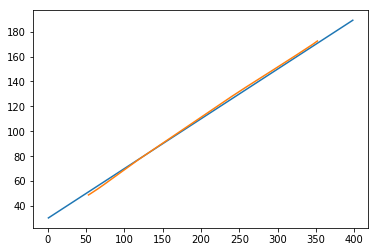
Now let’s see what our predictions look like.

现在，让我们看看我们的预测是什么样的。

In [408]:

在[408]中：

plt.plot(testx.reshape(398,2)[:,0:1], testx.reshape(398,2)[:,1:2])
plt.plot(predict[:,0:1], predict[:,1:2])

Out[408]:

出[408]：

[<matplotlib.lines.Line2D at 0x1eac792f048>]

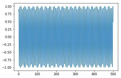
Now, we should try and model a sine or cosine wave in a similar fashion. You can run the code given below and play with the model parameters to see how the results change.

现在，我们应该尝试以类似方式对正弦波或余弦波建模。 您可以运行下面给出的代码，并使用模型参数来查看结果如何变化。

In [409]:

在[409]中：

x = numpy.arange (1,500,1)
y = numpy.sin(x)
plt.plot(x,y)

Out[409]:

出[409]：

[<matplotlib.lines.Line2D at 0x1eac7a0b3c8>]

In [410]:

在[410]中：

trainx, testx = x[0:int(0.8*(len(x)))], x[int(0.8*(len(x))):]
trainy, testy = y[0:int(0.8*(len(y)))], y[int(0.8*(len(y))):]
train = numpy.array(list(zip(trainx,trainy)))
test = numpy.array(list(zip(trainx,trainy)))

In [411]:

在[411]中：

look_back = 1
trainx,trainy = create_dataset(train, look_back)
testx,testy = create_dataset(test, look_back)

trainx = numpy.reshape(trainx, (trainx.shape[0], 1, 2))
testx = numpy.reshape(testx, (testx.shape[0], 1, 2))

In [ ]:

在[]中：

model = Sequential()
model.add(LSTM(512, return_sequences = True, input_shape = (trainx.shape[1], 2)))
model.add(LSTM(256,input_shape = (trainx.shape[1], 2)))
model.add(Dense(2))
model.compile(loss = 'mean_squared_error', optimizer = 'adam')
model.fit(trainx, trainy, epochs = 2000, batch_size = 10, verbose = 2, shuffle = False)
model.save_weights('LSTMBasic2.h5')

In [413]:

在[413]中：

model.load_weights('LSTMBasic2.h5')
predict = model.predict(testx)

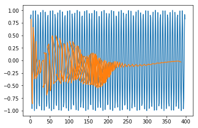
In [415]:

在[415]中：

plt.plot(trainx.reshape(398,2)[:,0:1], trainx.reshape(398,2)[:,1:2])
plt.plot(predict[:,0:1], predict[:,1:2])

Out [415]:

出[415]：

[<matplotlib.lines.Line2D at 0x1eac7a1f550>]

Now you are ready to move on to any dataset.

现在您可以继续使用任何数据集了。

翻译自: https://www.tutorialspoint.com/time_series/time_series_lstm_model.htm

lstm时间序列预测模型