LSTM时间序列预测及网络层搭建[通俗易懂]

大家好，又见面了，我是你们的朋友全栈君。

最近看到一篇博客，是时间预测问题，数据和代码的原地址在这里，
https://www.jianshu.com/p/5d6d5aac4dbd

下面只是对其复现和思考：
首先关于数据预处理的问题，大家可以参考：https://blog.csdn.net/lilong117194/article/details/82911073

1. LSTM预测未来一年某航空公司的客运流量

这里的问题是：给你一个数据集，只有一列数据，这是一个关于时间序列的数据，从这个时间序列中预测未来一年某航空公司的客运流量。
数据形式：

time passengers 0 1949-01 112 1 1949-02 118 2 1949-03 132 3 1949-04 129 4 1949-05 121 5 1949-06 135 6 1949-07 148 7 1949-08 148 8 1949-09 136 9 1949-10 119 ... ... .... 

下面的代码主要分为以下几步：

1. LSTM数据预处理
2. 搭建LSTM模型训练
3. 模型预测

数据预处理这块参考上面的链接就可以，而模型的搭建是基于keras的模型，稍微有点疑惑的地方就是数据的构建(训练集和测试集)，还有数据的预处理方法的问题。

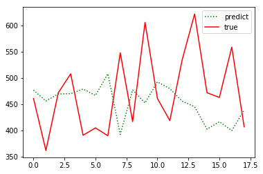
# -*- coding: utf-8 -*- import pandas as pd import numpy as np import matplotlib.pyplot as plt from sklearn.preprocessing import MinMaxScaler from keras.models import Sequential from keras.layers import LSTM, Dense, Activation def load_data(file_name, sequence_length=10, split=0.8): # 提取数据一列 df = pd.read_csv(file_name, sep=',', usecols=[1]) # 把数据转换为数组 data_all = np.array(df).astype(float) # 将数据缩放至给定的最小值与最大值之间，这里是０与１之间，数据预处理 scaler = MinMaxScaler() data_all = scaler.fit_transform(data_all) print(len(data_all)) data = [] # 构造送入lstm的3D数据：(133, 11, 1) for i in range(len(data_all) - sequence_length - 1): data.append(data_all[i: i + sequence_length + 1]) reshaped_data = np.array(data).astype('float64') print(reshaped_data.shape) # 打乱第一维的数据 np.random.shuffle(reshaped_data) print('reshaped_data:',reshaped_data[0]) # 这里对133组数据进行处理，每组11个数据中的前10个作为样本集：(133, 10, 1) x = reshaped_data[:, :-1] print('samples:',x.shape) # 133组样本中的每11个数据中的第11个作为样本标签 y = reshaped_data[:, -1] print('labels:',y.shape) # 构建训练集(训练集占了80%) split_boundary = int(reshaped_data.shape[0] * split) train_x = x[: split_boundary] # 构建测试集(原数据的后20%) test_x = x[split_boundary:] # 训练集标签 train_y = y[: split_boundary] # 测试集标签 test_y = y[split_boundary:] # 返回处理好的数据 return train_x, train_y, test_x, test_y, scaler # 模型建立 def build_model(): # input_dim是输入的train_x的最后一个维度，train_x的维度为(n_samples, time_steps, input_dim) model = Sequential() model.add(LSTM(input_dim=1, output_dim=50, return_sequences=True)) print(model.layers) model.add(LSTM(100, return_sequences=False)) model.add(Dense(output_dim=1)) model.add(Activation('linear')) model.compile(loss='mse', optimizer='rmsprop') return model def train_model(train_x, train_y, test_x, test_y): model = build_model() try: model.fit(train_x, train_y, batch_size=512, nb_epoch=30, validation_split=0.1) predict = model.predict(test_x) predict = np.reshape(predict, (predict.size, )) except KeyboardInterrupt: print(predict) print(test_y) print('predict:\n',predict) print('test_y:\n',test_y) # 预测的散点值和真实的散点值画图 try: fig1 = plt.figure(1) plt.plot(predict, 'r:') plt.plot(test_y, 'g-') plt.legend(['predict', 'true']) except Exception as e: print(e) return predict, test_y if __name__ == '__main__': # 加载数据 train_x, train_y, test_x, test_y, scaler = load_data('international-airline-passengers.csv') train_x = np.reshape(train_x, (train_x.shape[0], train_x.shape[1], 1)) test_x = np.reshape(test_x, (test_x.shape[0], test_x.shape[1], 1)) # 模型训练  predict_y, test_y = train_model(train_x, train_y, test_x, test_y) # 对标准化处理后的数据还原 predict_y = scaler.inverse_transform([[i] for i in predict_y]) test_y = scaler.inverse_transform(test_y) # 把预测和真实数据对比 fig2 = plt.figure(2) plt.plot(predict_y, 'g:') plt.plot(test_y, 'r-') plt.legend(['predict', 'true']) plt.show() 

运行结果：

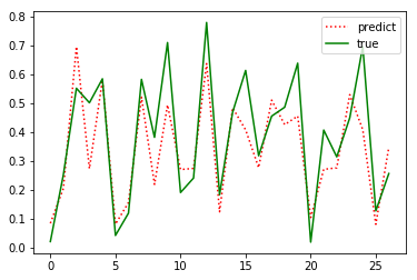
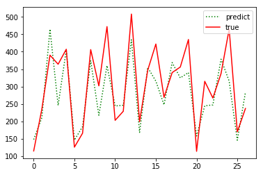
从结果可以看出预测效果还可以，但是理论上存在诸多问题：

1. 在normalize data的时候，直接拿所有的data， data_all 去normalize, 但合理的做法应该是normalize train, 然后用train的parameter 去normalize test。因为用整个data set 去normalize 的话相当于提前获取了未来的信息。
2. 就是源代码中的打乱数据顺序，本质上造成了历史和未来的混淆，实际是用到了未来的数据预测趋势，overfitting了。

基于以上的主要问题，在完全没有未来数据参与下进行训练，进行修改后的数据处理过程如下：全集—分割—训练集归一训练—验证集使用训练集std&mean进行归一完成预测。

这里就是先试下没有打乱数据的情况，就是按照顺序的数据集构建进行训练和预测：

#!/usr/bin/env python3 # -*- coding: utf-8 -*- import pandas as pd import numpy as np import matplotlib.pyplot as plt from sklearn.preprocessing import MinMaxScaler from keras.models import Sequential from keras.layers import LSTM, Dense, Activation # 数据集的构建 def dataset_func(data_pro,sequence_length=10): data = [] # 构造数据集：构造送入lstm的3D数据 for i in range(len(data_pro) - sequence_length - 1): data.append(data_pro[i: i + sequence_length + 1]) reshaped_data = np.array(data).astype('float64') print('here:',reshaped_data.shape) # 打乱数据集 #np.random.shuffle(reshaped_data) print('reshaped_data:',reshaped_data[0]) # 数据集的特征和标签分开：样本中的每11个数据中的第11个作为样本标签 x = reshaped_data[:, :-1] print('samples:',x.shape) y = reshaped_data[:, -1] print('labels:',y.shape) return x,y def load_data(file_name, sequence_length=10, split=0.8): # 提取数据一列 df = pd.read_csv(file_name, sep=',', usecols=[1]) # 把数据转换为数组 data_all = np.array(df).astype(float) print('length of data_all:',data_all.shape) # 全集划分：80%的训练数据 split_boundary = int(data_all.shape[0] * split) print(split_boundary) train_x = data_all[: split_boundary] print(train_x.shape) # 训练集的归一化:将数据缩放至给定的最小值与最大值之间，这里是０与１之间，数据预处理 scaler = MinMaxScaler() data_train = scaler.fit_transform(train_x) print('length:',len(data_train)) train_x,train_y=dataset_func(data_train,sequence_length=10) # 全集划分：20%的验证数据 test_x = data_all[split_boundary:] print(test_x.shape) data_test = scaler.transform(test_x) print('length:',len(data_test)) test_x,test_y=dataset_func(data_test,sequence_length=10) # 返回处理好的数据 return train_x, train_y, test_x, test_y, scaler # 模型建立 def build_model(): # input_dim是输入的train_x的最后一个维度，train_x的维度为(n_samples, time_steps, input_dim) model = Sequential() model.add(LSTM(input_dim=1, output_dim=50, return_sequences=True)) print(model.layers) model.add(LSTM(100, return_sequences=False)) model.add(Dense(output_dim=1)) model.add(Activation('linear')) model.compile(loss='mse', optimizer='rmsprop') return model def train_model(train_x, train_y, test_x, test_y): model = build_model() try: model.fit(train_x, train_y, batch_size=512, nb_epoch=30, validation_split=0.1) predict = model.predict(test_x) predict = np.reshape(predict, (predict.size, )) except KeyboardInterrupt: print(predict) print(test_y) print('predict:\n',predict) print('test_y:\n',test_y) # 预测的散点值和真实的散点值画图 try: fig1 = plt.figure(1) plt.plot(predict, 'r:') plt.plot(test_y, 'g-') plt.legend(['predict', 'true']) except Exception as e: print(e) return predict, test_y if __name__ == '__main__': # 加载数据 train_x, train_y, test_x, test_y, scaler = load_data('international-airline-passengers.csv') train_x = np.reshape(train_x, (train_x.shape[0], train_x.shape[1], 1)) test_x = np.reshape(test_x, (test_x.shape[0], test_x.shape[1], 1)) # 模型训练  predict_y, test_y = train_model(train_x, train_y, test_x, test_y) # 对标准化处理后的数据还原 predict_y = scaler.inverse_transform([[i] for i in predict_y]) test_y = scaler.inverse_transform(test_y) # 把预测和真实数据对比 fig2 = plt.figure(2) plt.plot(predict_y, 'g:') plt.plot(test_y, 'r-') plt.legend(['predict', 'true']) plt.show() 

主要就是数据的构建改变了，运行结果如下：

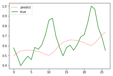
可以看出效果很差，具体为什么按照常规的顺序数据构建（不打乱）预测效果那么差，还在思考中。。。。

下面又尝试了：全集—分割—训练集归一shuffle并记录std&mean—训练—验证集使用训练集std&mean进行归一完成预测。
仅仅把上面代码中数据顺序打乱的注释去掉就可以了：
#np.random.shuffle(reshaped_data)
再次训练得到：

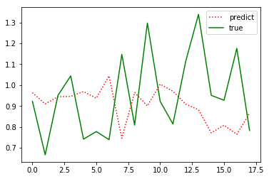
效果还是不理想，所以这里仅仅作为学习的过程，以后再研究。

2. keras的lstm层函数

keras.layers.recurrent.LSTM(units, activation='tanh', recurrent_activation='hard_sigmoid', use_bias=True, kernel_initializer='glorot_uniform', recurrent_initializer='orthogonal', bias_initializer='zeros', unit_forget_bias=True, kernel_regularizer=None, recurrent_regularizer=None, bias_regularizer=None, activity_regularizer=None, kernel_constraint=None, recurrent_constraint=None, bias_constraint=None, dropout=0.0, recurrent_dropout=0.0)

2.1 参数说明：

• units：输出维度
• input_dim：输入维度，当使用该层为模型首层时，应指定该值（或等价的指定input_shape)
• return_sequences：布尔值，默认False，控制返回类型。若为True则返回整个序列，否则仅返回输出序列的最后一个输出
• input_length：当输入序列的长度固定时，该参数为输入序列的长度。当需要在该层后连接Flatten层，然后又要连接Dense层时，需要指定该参数，否则全连接的输出无法计算出来。

2.2 输入shape ：

形如（samples，timesteps，input_dim）的3D张量

2.3 输出shape：

如果return_sequences=True：返回形如（samples，timesteps，output_dim）的3D张量，否则返回形如（samples，output_dim）的2D张量。

2.4 输入和输出的类型 ：

相对之前的tensor，这里多了个参数timesteps，其表示什么意思？假如我们输入有100个句子，每个句子都由5个单词组成，而每个单词用64维的词向量表示。那么samples=100，timesteps=5，input_dim=64，可以简单地理解timesteps就是输入序列的长度input_length(视情而定)

2.5 units ：

假如units=128，就一个单词而言，你可以把LSTM内部简化看成 :
$Y=X_{1\times 64}{W}_{64\times 128}$,X为上面提及的词向量比如64维,W中的128就是units，也就是说通过LSTM，把词的维度由64转变成了128

2.6 return_sequences

我们可以把很多LSTM层串在一起，但是最后一个LSTM层return_sequences通常为false，具体看下面的例子：
句子：you are really a genius

model = Sequential()
model.add(LSTM(128, input_dim=64, input_length=5, return_sequences=True))
model.add(LSTM(256, return_sequences=False))

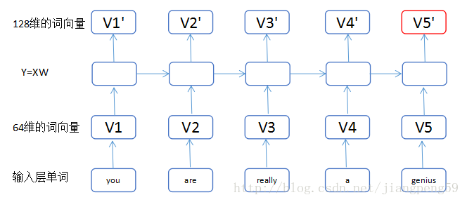
(1)我们把输入的单词，转换为维度64的词向量，最下面一层的小矩形的数目即单词的个数input_length（每个句子的单词个数）。
(2)通过第一个LSTM中的Y=XW，这里输入为维度64，输出为维度128，而return_sequences=True，我们可以获得5个128维的词向量$V{1}^{\prime },V2...V{5}^{\prime }$
(3)通过第二个LSTM（这里上图没有显示出来，最上面应该还有一层），此时输入为$V{1}^{\prime },V2...V{5}^{\prime }$都为128维，经转换后得到$V{1}^{\prime \prime },V{2}^{\prime \prime },...V{5}^{\prime \prime }$为256维，最后因为return_sequences=False，所以只输出了最后一个红色的词向量。

下面是一个动态图，有助于理解：

2.7 在实际应用中，有如下的表示形式：

1. 输入维度   input_dim=1
2. 输出维度   output_dim=6
3. 滑动窗口  input_length=10

model.add(LSTM(input_dim=1, output_dim=6,input_length=10, return_sequences=True)) model.add(LSTM(6, input_dim=1, input_length=10, return_sequences=True)) model.add(LSTM(6, input_shape=(10, 1),return_sequences=True)) 

参考：
https://www.zhihu.com/question/41949741?sort=created
https://blog.csdn.net/jiangpeng59/article/details/77646186