faster rcnn 详解

转自：https://zhuanlan.zhihu.com/p/31426458

经过R-CNN和Fast RCNN的积淀，Ross B. Girshick在2016年提出了新的Faster RCNN，在结构上，Faster RCNN已经将特征抽取(feature extraction)，proposal提取，bounding box regression(rect refine)，classification都整合在了一个网络中，使得综合性能有较大提高，在检测速度方面尤为明显。

&lt;img src=”https://pic4.zhimg.com/v2-c0172be282021a1029f7b72b51079ffe_b.jpg” data-size=”normal” data-rawwidth=”408″ data-rawheight=”407″ class=”content_image” width=”408″&gt;

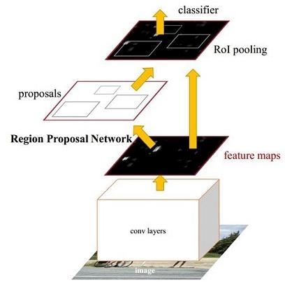
faster rcnn 详解图1 Faster RCNN基本结构（来自原论文）

依作者看来，如图1，Faster RCNN其实可以分为4个主要内容：

Conv layers。作为一种CNN网络目标检测方法，Faster RCNN首先使用一组基础的conv+relu+pooling层提取image的feature maps。该feature maps被共享用于后续RPN层和全连接层。
Region Proposal Networks。RPN网络用于生成region proposals。该层通过softmax判断anchors属于foreground或者background，再利用bounding box regression修正anchors获得精确的proposals。
Roi Pooling。该层收集输入的feature maps和proposals，综合这些信息后提取proposal feature maps，送入后续全连接层判定目标类别。
Classification。利用proposal feature maps计算proposal的类别，同时再次bounding box regression获得检测框最终的精确位置。

所以本文以上述4个内容作为切入点介绍Faster R-CNN网络。
图2展示了python版本中的VGG16模型中的faster_rcnn_test.pt的网络结构，可以清晰的看到该网络对于一副任意大小PxQ的图像，首先缩放至固定大小MxN，然后将MxN图像送入网络；而Conv layers中包含了13个conv层+13个relu层+4个pooling层；RPN网络首先经过3×3卷积，再分别生成foreground anchors与bounding box regression偏移量，然后计算出proposals；而Roi Pooling层则利用proposals从feature maps中提取proposal feature送入后续全连接和softmax网络作classification（即分类proposal到底是什么object）。

&lt;img src=”https://pic1.zhimg.com/v2-e64a99b38f411c337f538eb5f093bdf3_b.jpg” data-size=”normal” data-rawwidth=”965″ data-rawheight=”472″ class=”origin_image zh-lightbox-thumb” width=”965″ data-original=”https://pic1.zhimg.com/v2-e64a99b38f411c337f538eb5f093bdf3_r.jpg”&gt;

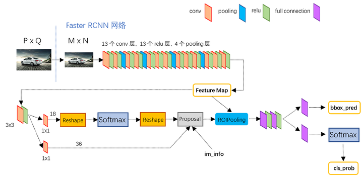图2 faster_rcnn_test.pt网络结构（pascal_voc/VGG16/faster_rcnn_alt_opt/faster_rcnn_test.pt）

本文不会讨论任何关于R-CNN家族的历史，分析清楚最新的Faster R-CNN就够了，并不需要追溯到那么久。实话说我也不了解R-CNN，更不关心。有空不如看看新算法。

1 Conv layers

Conv layers包含了conv，pooling，relu三种层。以python版本中的VGG16模型中的faster_rcnn_test.pt的网络结构为例，如图2，Conv layers部分共有13个conv层，13个relu层，4个pooling层。这里有一个非常容易被忽略但是又无比重要的信息，在Conv layers中：

所有的conv层都是： $kernel\_size=3$ ，，
所有的pooling层都是： $kernel\_size=2$ ，，

为何重要？在Faster RCNN Conv layers中对所有的卷积都做了扩边处理（ pad=1，即填充一圈0），导致原图变为 (M+2)x(N+2)大小，再做3×3卷积后输出MxN 。正是这种设置，导致Conv layers中的conv层不改变输入和输出矩阵大小。如图3：

&lt;img src=”https://pic3.zhimg.com/v2-3c772e9ed555eb86a97ef9c08bf563c9_b.jpg” data-size=”normal” data-rawwidth=”787″ data-rawheight=”300″ class=”origin_image zh-lightbox-thumb” width=”787″ data-original=”https://pic3.zhimg.com/v2-3c772e9ed555eb86a97ef9c08bf563c9_r.jpg”&gt;

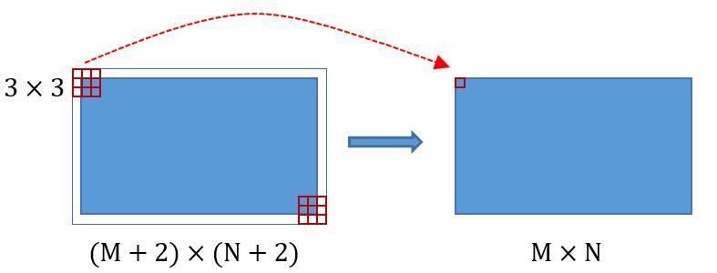图3 卷积示意图

类似的是，Conv layers中的pooling层kernel_size=2，stride=2。这样每个经过pooling层的MxN矩阵，都会变为(M/2)x(N/2)大小。综上所述，在整个Conv layers中，conv和relu层不改变输入输出大小，只有pooling层使输出长宽都变为输入的1/2。
那么，一个MxN大小的矩阵经过Conv layers固定变为(M/16)x(N/16)！这样Conv layers生成的featuure map中都可以和原图对应起来。

2 Region Proposal Networks(RPN)

经典的检测方法生成检测框都非常耗时，如OpenCV adaboost使用滑动窗口+图像金字塔生成检测框；或如R-CNN使用SS(Selective Search)方法生成检测框。而Faster RCNN则抛弃了传统的滑动窗口和SS方法，直接使用RPN生成检测框，这也是Faster R-CNN的巨大优势，能极大提升检测框的生成速度。

&lt;img src=”https://pic4.zhimg.com/v2-1908feeaba591d28bee3c4a754cca282_b.jpg” data-size=”normal” data-rawwidth=”843″ data-rawheight=”219″ class=”origin_image zh-lightbox-thumb” width=”843″ data-original=”https://pic4.zhimg.com/v2-1908feeaba591d28bee3c4a754cca282_r.jpg”&gt;

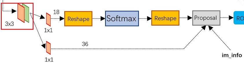图4 RPN网络结构

上图4展示了RPN网络的具体结构。可以看到RPN网络实际分为2条线，上面一条通过softmax分类anchors获得foreground和background（检测目标是foreground），下面一条用于计算对于anchors的bounding box regression偏移量，以获得精确的proposal。而最后的Proposal层则负责综合foreground anchors和bounding box regression偏移量获取proposals，同时剔除太小和超出边界的proposals。其实整个网络到了Proposal Layer这里，就完成了相当于目标定位的功能。

2.1 多通道图像卷积基础知识介绍

在介绍RPN前，还要多解释几句基础知识，已经懂的看官老爷跳过就好。

对于单通道图像+单卷积核做卷积，第一章中的图3已经展示了；
对于多通道图像+多卷积核做卷积，计算方式如下：

&lt;img src=”https://pic4.zhimg.com/v2-8d72777321cbf1336b79d839b6c7f9fc_b.jpg” data-size=”normal” data-rawwidth=”842″ data-rawheight=”456″ class=”origin_image zh-lightbox-thumb” width=”842″ data-original=”https://pic4.zhimg.com/v2-8d72777321cbf1336b79d839b6c7f9fc_r.jpg”&gt;

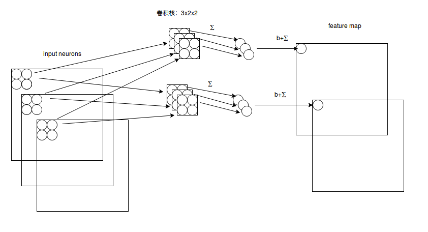图5 多通道卷积计算方式

如图5，输入有3个通道，同时有2个卷积核。对于每个卷积核，先在输入3个通道分别作卷积，再将3个通道结果加起来得到卷积输出。所以对于某个卷积层，无论输入图像有多少个通道，输出图像通道数总是等于卷积核数量！
对多通道图像做1×1卷积，其实就是将输入图像于每个通道乘以卷积系数后加在一起，即相当于把原图像中本来各个独立的通道“联通”在了一起。

2.2 anchors

提到RPN网络，就不能不说anchors。所谓anchors，实际上就是一组由rpn/generate_anchors.py生成的矩形。直接运行作者demo中的generate_anchors.py可以得到以下输出：

[[ -84.  -40.   99.   55.]
 [-176.  -88.  191.  103.]
 [-360. -184.  375.  199.]
 [ -56.  -56.   71.   71.]
 [-120. -120.  135.  135.]
 [-248. -248.  263.  263.]
 [ -36.  -80.   51.   95.]
 [ -80. -168.   95.  183.]
 [-168. -344.  183.  359.]]

其中每行的4个值(x1, y1, x2, y2) 表矩形左上和右下角点坐标。9个矩形共有3种形状，长宽比为大约为with:height∈{1:1, 1:2, 2:1}三种，如图6。实际上通过anchors就引入了检测中常用到的多尺度方法。

&lt;img src=”https://pic1.zhimg.com/v2-7abead97efcc46a3ee5b030a2151643f_b.jpg” data-size=”normal” data-rawwidth=”253″ data-rawheight=”245″ class=”content_image” width=”253″&gt;

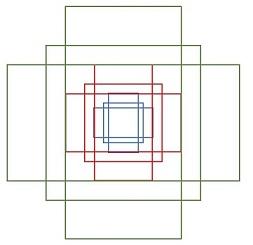图6 anchors示意图

注：关于上面的anchors size，其实是根据检测图像设置的。在python demo中，会把任意大小的输入图像reshape成800×600（即图2中的M=800，N=600）。再回头来看anchors的大小，anchors中长宽1:2中最大为352×704，长宽2:1中最大736×384，基本是cover了800×600的各个尺度和形状。
那么这9个anchors是做什么的呢？借用Faster RCNN论文中的原图，如图7，遍历Conv layers计算获得的feature maps，为每一个点都配备这9种anchors作为初始的检测框。这样做获得检测框很不准确，不用担心，后面还有2次bounding box regression可以修正检测框位置。

&lt;img src=”https://pic3.zhimg.com/v2-c93db71cc8f4f4fd8cfb4ef2e2cef4f4_b.jpg” data-size=”normal” data-rawwidth=”418″ data-rawheight=”241″ class=”content_image” width=”418″&gt;

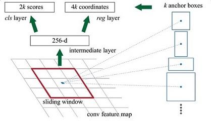图7

解释一下上面这张图的数字。

在原文中使用的是ZF model中，其Conv Layers中最后的conv5层num_output=256，对应生成256张特征图，所以相当于feature map每个点都是256-dimensions
在conv5之后，做了rpn_conv/3×3卷积且num_output=256，相当于每个点又融合了周围3×3的空间信息（猜测这样做也许更鲁棒？反正我没测试），同时256-d不变（如图4和图7中的红框）
假设在conv5 feature map中每个点上有k个anchor（默认k=9），而每个anhcor要分foreground和background，所以每个点由256d feature转化为cls=2k scores；而每个anchor都有[x, y, w, h]对应4个偏移量，所以reg=4k coordinates
补充一点，全部anchors拿去训练太多了，训练程序会在合适的anchors中随机选取128个postive anchors+128个negative anchors进行训练（什么是合适的anchors下文5.1有解释）

注意，在本文讲解中使用的VGG conv5 num_output=512，所以是512d，其他类似。

其实RPN最终就是在原图尺度上，设置了密密麻麻的候选Anchor。然后用cnn去判断哪些Anchor是里面有目标的foreground anchor，哪些是没目标的backgroud。所以，仅仅是个二分类而已！

那么Anchor一共有多少个？原图800×600，VGG下采样16倍，feature map每个点设置9个Anchor，所以：

$ceil(800/16) \times ceil(600/16) \times 9=50\times38 \times9=17100$

其中ceil()表示向上取整，是因为VGG输出的feature map size= 50*38。

&lt;img src=”https://pic2.zhimg.com/v2-4b15828dfee19be726835b671748cc4d_b.jpg” data-size=”normal” data-rawwidth=”1223″ data-rawheight=”776″ class=”origin_image zh-lightbox-thumb” width=”1223″ data-original=”https://pic2.zhimg.com/v2-4b15828dfee19be726835b671748cc4d_r.jpg”&gt;

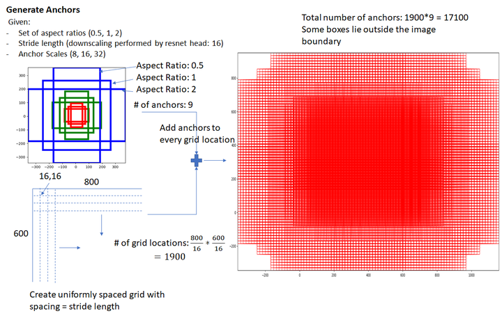图8 Gernerate Anchors

看官老爷们，这还不懂？再问Anchor怎么来的直播跳楼！

2.3 softmax判定foreground与background

一副MxN大小的矩阵送入Faster RCNN网络后，到RPN网络变为(M/16)x(N/16)，不妨设 W=M/16，H=N/16。在进入reshape与softmax之前，先做了1×1卷积，如图9：

&lt;img src=”https://pic1.zhimg.com/v2-1ab4b6c3dd607a5035b5203c76b078f3_b.jpg” data-size=”normal” data-rawwidth=”713″ data-rawheight=”123″ class=”origin_image zh-lightbox-thumb” width=”713″ data-original=”https://pic1.zhimg.com/v2-1ab4b6c3dd607a5035b5203c76b078f3_r.jpg”&gt;

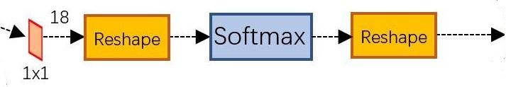图9 RPN中判定fg/bg网络结构

该1×1卷积的caffe prototxt定义如下：

layer {
  name: "rpn_cls_score"
  type: "Convolution"
  bottom: "rpn/output"
  top: "rpn_cls_score"
  convolution_param {
    num_output: 18   # 2(bg/fg) * 9(anchors)
    kernel_size: 1 pad: 0 stride: 1
  }
}

可以看到其num_output=18，也就是经过该卷积的输出图像为WxHx18大小（注意第二章开头提到的卷积计算方式）。这也就刚好对应了feature maps每一个点都有9个anchors，同时每个anchors又有可能是foreground和background，所有这些信息都保存WxHx(9*2)大小的矩阵。为何这样做？后面接softmax分类获得foreground anchors，也就相当于初步提取了检测目标候选区域box（一般认为目标在foreground anchors中）。
那么为何要在softmax前后都接一个reshape layer？其实只是为了便于softmax分类，至于具体原因这就要从caffe的实现形式说起了。在caffe基本数据结构blob中以如下形式保存数据：

blob=[batch_size, channel，height，width]

对应至上面的保存bg/fg anchors的矩阵，其在caffe blob中的存储形式为[1, 2×9, H, W]。而在softmax分类时需要进行fg/bg二分类，所以reshape layer会将其变为[1, 2, 9xH, W]大小，即单独“腾空”出来一个维度以便softmax分类，之后再reshape回复原状。贴一段caffe softmax_loss_layer.cpp的reshape函数的解释，非常精辟：

"Number of labels must match number of predictions; " "e.g., if softmax axis == 1 and prediction shape is (N, C, H, W), " "label count (number of labels) must be N*H*W, " "with integer values in {0, 1, ..., C-1}.";

综上所述，RPN网络中利用anchors和softmax初步提取出foreground anchors作为候选区域。

2.4 bounding box regression原理

如图9所示绿色框为飞机的Ground Truth(GT)，红色为提取的foreground anchors，即便红色的框被分类器识别为飞机，但是由于红色的框定位不准，这张图相当于没有正确的检测出飞机。所以我们希望采用一种方法对红色的框进行微调，使得foreground anchors和GT更加接近。

&lt;img src=”https://pic3.zhimg.com/v2-93021a3c03d66456150efa1da95416d3_b.jpg” data-size=”normal” data-rawwidth=”305″ data-rawheight=”232″ class=”content_image” width=”305″&gt;

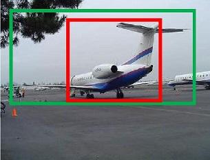图10

对于窗口一般使用四维向量 (x, y, w, h)表示，分别表示窗口的中心点坐标和宽高。对于图 11，红色的框A代表原始的Foreground Anchors，绿色的框G代表目标的GT，我们的目标是寻找一种关系，使得输入原始的anchor A经过映射得到一个跟真实窗口G更接近的回归窗口G’，即：

给定：anchor $A=(A_{x}, A_{y}, A_{w}, A_{h})$ 和 $GT=[G_{x}, G_{y}, G_{w}, G_{h}]$
寻找一种变换F，使得： $F(A_{x}, A_{y}, A_{w}, A_{h})=(G_{x}^{'}, G_{y}^{'}, G_{w}^{'}, G_{h}^{'})$ ，其中 $(G_{x}^{'}, G_{y}^{'}, G_{w}^{'}, G_{h}^{'})≈(G_{x}, G_{y}, G_{w}, G_{h})$

&lt;img src=”https://pic1.zhimg.com/v2-ea7e6e48662bfa68ec73bdf32f36bb85_b.jpg” data-size=”normal” data-rawwidth=”233″ data-rawheight=”218″ class=”content_image” width=”233″&gt;

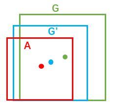图11

那么经过何种变换F才能从图10中的anchor A变为G’呢？比较简单的思路就是:

先做平移

&lt;img src=”https://pic1.zhimg.com/v2-a9380736b49a548736b35d182ffd44ab_b.jpg” data-caption=”” data-size=”normal” data-rawwidth=”215″ data-rawheight=”63″ class=”content_image” width=”215″&gt;

再做缩放

&lt;img src=”https://pic1.zhimg.com/v2-c4d9c89c3fb1baa90631f662f906626f_b.jpg” data-caption=”” data-size=”normal” data-rawwidth=”215″ data-rawheight=”64″ class=”content_image” width=”215″&gt;

观察上面4个公式发现，需要学习的是 $d_{x}(A),d_{y}(A),d_{w}(A),d_{h}(A)$ 这四个变换。当输入的anchor A与GT相差较小时，可以认为这种变换是一种线性变换，那么就可以用线性回归来建模对窗口进行微调（注意，只有当anchors A和GT比较接近时，才能使用线性回归模型，否则就是复杂的非线性问题了）。
接下来的问题就是如何通过线性回归获得 $d_{x}(A),d_{y}(A),d_{w}(A),d_{h}(A)$ 了。线性回归就是给定输入的特征向量X, 学习一组参数W, 使得经过线性回归后的值跟真实值Y非常接近，即。对于该问题，输入X是cnn feature map，定义为Φ；同时还有训练传入A与GT之间的变换量，即 $(t_{x}, t_{y}, t_{w}, t_{h})$ 。输出是 $d_{x}(A),d_{y}(A),d_{w}(A),d_{h}(A)$ 四个变换。那么目标函数可以表示为：

&lt;img src=”https://pic4.zhimg.com/v2-0dad3f869b9c1760c7188efd0b6f81f1_b.jpg” data-caption=”” data-size=”normal” data-rawwidth=”203″ data-rawheight=”37″ class=”content_image” width=”203″&gt;

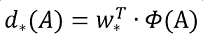
其中Φ(A)是对应anchor的feature map组成的特征向量，w是需要学习的参数，d(A)是得到的预测值（*表示 x，y，w，h，也就是每一个变换对应一个上述目标函数）。为了让预测值 $(t_{x}, t_{y}, t_{w}, t_{h})$ 与真实值差距最小，设计损失函数：

&lt;img src=”https://pic4.zhimg.com/v2-c898fc9738b82afa2729a5a5f61ac893_b.jpg” data-caption=”” data-size=”normal” data-rawwidth=”274″ data-rawheight=”70″ class=”content_image” width=”274″&gt;

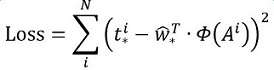
函数优化目标为：

&lt;img src=”https://pic1.zhimg.com/v2-1e67089e47548f8a383a221f184dea04_b.jpg” data-caption=”” data-size=”normal” data-rawwidth=”405″ data-rawheight=”69″ class=”content_image” width=”405″&gt;

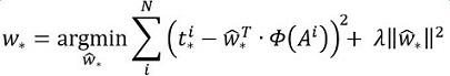
需要说明，只有在GT与需要回归框位置比较接近时，才可近似认为上述线性变换成立。
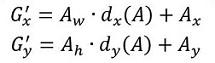
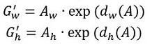
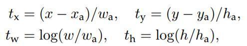
说完原理，对应于Faster RCNN原文，foreground anchor与ground truth之间的平移量与尺度因子如下：

&lt;img src=”https://pic4.zhimg.com/v2-18fdc24fc392a80e456b77b9a7f69c71_b.jpg” data-caption=”” data-size=”normal” data-rawwidth=”495″ data-rawheight=”92″ class=”origin_image zh-lightbox-thumb” width=”495″ data-original=”https://pic4.zhimg.com/v2-18fdc24fc392a80e456b77b9a7f69c71_r.jpg”&gt;

对于训练bouding box regression网络回归分支，输入是cnn feature Φ，监督信号是Anchor与GT的差距，即训练目标是：输入 Φ的情况下使网络输出与监督信号尽可能接近。
那么当bouding box regression工作时，再输入Φ时，回归网络分支的输出就是每个Anchor的平移量和变换尺度，显然即可用来修正Anchor位置了。

2.5 对proposals进行bounding box regression

在了解bounding box regression后，再回头来看RPN网络第二条线路，如图12。

&lt;img src=”https://pic4.zhimg.com/v2-8241c8076d60156248916fe2f1a5674a_b.jpg” data-size=”normal” data-rawwidth=”693″ data-rawheight=”126″ class=”origin_image zh-lightbox-thumb” width=”693″ data-original=”https://pic4.zhimg.com/v2-8241c8076d60156248916fe2f1a5674a_r.jpg”&gt;

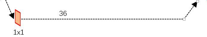图12 RPN中的bbox reg

先来看一看上图11中1×1卷积的caffe prototxt定义：

layer {
  name: "rpn_bbox_pred"
  type: "Convolution"
  bottom: "rpn/output"
  top: "rpn_bbox_pred"
  convolution_param {
    num_output: 36   # 4 * 9(anchors)
    kernel_size: 1 pad: 0 stride: 1
  }
}

可以看到其 num_output=36，即经过该卷积输出图像为WxHx36，在caffe blob存储为[1, 4×9, H, W]，这里相当于feature maps每个点都有9个anchors，每个anchors又都有4个用于回归的 $[d_{x}(A),d_{y}(A),d_{w}(A),d_{h}(A)]$ 变换量。

2.6 Proposal Layer

Proposal Layer负责综合所有 $[d_{x}(A),d_{y}(A),d_{w}(A),d_{h}(A)]$ 变换量和foreground anchors，计算出精准的proposal，送入后续RoI Pooling Layer。还是先来看看Proposal Layer的caffe prototxt定义：

layer {
  name: 'proposal'
  type: 'Python'
  bottom: 'rpn_cls_prob_reshape'
  bottom: 'rpn_bbox_pred'
  bottom: 'im_info'
  top: 'rois'
  python_param {
    module: 'rpn.proposal_layer'
    layer: 'ProposalLayer'
    param_str: "'feat_stride': 16"
  }
}

Proposal Layer有3个输入：fg/bg anchors分类器结果rpn_cls_prob_reshape，对应的bbox reg的 $[d_{x}(A),d_{y}(A),d_{w}(A),d_{h}(A)]$ 变换量rpn_bbox_pred，以及im_info；另外还有参数feat_stride=16，这和图4是对应的。
首先解释im_info。对于一副任意大小PxQ图像，传入Faster RCNN前首先reshape到固定MxN，im_info=[M, N, scale_factor]则保存了此次缩放的所有信息。然后经过Conv Layers，经过4次pooling变为WxH=(M/16)x(N/16)大小，其中feature_stride=16则保存了该信息，用于计算anchor偏移量。

&lt;img src=”https://pic4.zhimg.com/v2-1e43500c7cc9a9de211d737bc347ced9_b.jpg” data-size=”normal” data-rawwidth=”792″ data-rawheight=”186″ class=”origin_image zh-lightbox-thumb” width=”792″ data-original=”https://pic4.zhimg.com/v2-1e43500c7cc9a9de211d737bc347ced9_r.jpg”&gt;

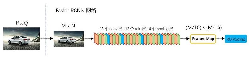图13

Proposal Layer forward（caffe layer的前传函数）按照以下顺序依次处理：

生成anchors，利用 $[d_{x}(A),d_{y}(A),d_{w}(A),d_{h}(A)]$ 对所有的anchors做bbox regression回归（这里的anchors生成和训练时完全一致）
按照输入的foreground softmax scores由大到小排序anchors，提取前pre_nms_topN(e.g. 6000)个anchors，即提取修正位置后的foreground anchors。
限定超出图像边界的foreground anchors为图像边界（防止后续roi pooling时proposal超出图像边界）
剔除非常小（width<threshold or height<threshold）的foreground anchors
进行nonmaximum suppression
再次按照nms后的foreground softmax scores由大到小排序fg anchors，提取前post_nms_topN(e.g. 300)结果作为proposal输出。

之后输出proposal=[x1, y1, x2, y2]，注意，由于在第三步中将anchors映射回原图判断是否超出边界，所以这里输出的proposal是对应MxN输入图像尺度的，这点在后续网络中有用。另外我认为，严格意义上的检测应该到此就结束了，后续部分应该属于识别了~
RPN网络结构就介绍到这里，总结起来就是：
生成anchors -> softmax分类器提取fg anchors -> bbox reg回归fg anchors -> Proposal Layer生成proposals

3 RoI pooling

而RoI Pooling层则负责收集proposal，并计算出proposal feature maps，送入后续网络。从图2中可以看到Rol pooling层有2个输入：

原始的feature maps
RPN输出的proposal boxes（大小各不相同）

3.1 为何需要RoI Pooling

先来看一个问题：对于传统的CNN（如AlexNet，VGG），当网络训练好后输入的图像尺寸必须是固定值，同时网络输出也是固定大小的vector or matrix。如果输入图像大小不定，这个问题就变得比较麻烦。有2种解决办法：

从图像中crop一部分传入网络
将图像warp成需要的大小后传入网络

&lt;img src=”https://pic2.zhimg.com/v2-e525342cbde476a11c48a6be393f226c_b.jpg” data-size=”normal” data-rawwidth=”896″ data-rawheight=”198″ class=”origin_image zh-lightbox-thumb” width=”896″ data-original=”https://pic2.zhimg.com/v2-e525342cbde476a11c48a6be393f226c_r.jpg”&gt;

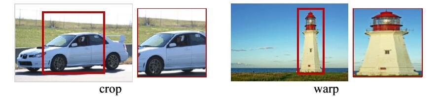图14 crop与warp破坏图像原有结构信息

两种办法的示意图如图14，可以看到无论采取那种办法都不好，要么crop后破坏了图像的完整结构，要么warp破坏了图像原始形状信息。
回忆RPN网络生成的proposals的方法：对foreground anchors进行bounding box regression，那么这样获得的proposals也是大小形状各不相同，即也存在上述问题。所以Faster R-CNN中提出了RoI Pooling解决这个问题。不过RoI Pooling确实是从Spatial Pyramid Pooling发展而来，但是限于篇幅这里略去不讲，有兴趣的读者可以自行查阅相关论文。

3.2 RoI Pooling原理

分析之前先来看看RoI Pooling Layer的caffe prototxt的定义：

layer {
  name: "roi_pool5"
  type: "ROIPooling"
  bottom: "conv5_3"
  bottom: "rois"
  top: "pool5"
  roi_pooling_param {
    pooled_w: 7
    pooled_h: 7
    spatial_scale: 0.0625 # 1/16
  }
}

其中有新参数，另外一个参数认真阅读的读者肯定已经知道知道用途。
RoI Pooling layer forward过程：在之前有明确提到：是对应MxN尺度的，所以首先使用spatial_scale参数将其映射回(M/16)x(N/16)大小的feature maps尺度；之后将每个proposal水平和竖直分为pooled_w和pooled_h份，对每一份都进行max pooling处理。这样处理后，即使大小不同的proposal，输出结果都是大小，实现了fixed-length output（固定长度输出）。

&lt;img src=”https://pic2.zhimg.com/v2-e3108dc5cdd76b871e21a4cb64001b5c_b.jpg” data-size=”normal” data-rawwidth=”615″ data-rawheight=”312″ class=”origin_image zh-lightbox-thumb” width=”615″ data-original=”https://pic2.zhimg.com/v2-e3108dc5cdd76b871e21a4cb64001b5c_r.jpg”&gt;

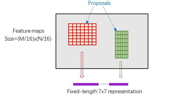图15 proposal示意图

4 Classification

Classification部分利用已经获得的proposal feature maps，通过full connect层与softmax计算每个proposal具体属于那个类别（如人，车，电视等），输出cls_prob概率向量；同时再次利用bounding box regression获得每个proposal的位置偏移量bbox_pred，用于回归更加精确的目标检测框。Classification部分网络结构如图16。

&lt;img src=”https://pic4.zhimg.com/v2-9377a45dc8393d546b7b52a491414ded_b.jpg” data-size=”normal” data-rawwidth=”669″ data-rawheight=”154″ class=”origin_image zh-lightbox-thumb” width=”669″ data-original=”https://pic4.zhimg.com/v2-9377a45dc8393d546b7b52a491414ded_r.jpg”&gt;

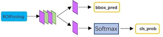图16 Classification部分网络结构图

从PoI Pooling获取到7×7=49大小的proposal feature maps后，送入后续网络，可以看到做了如下2件事：

通过全连接和softmax对proposals进行分类，这实际上已经是识别的范畴了
再次对proposals进行bounding box regression，获取更高精度的rect box

这里来看看全连接层InnerProduct layers，简单的示意图如图17，

&lt;img src=”https://pic4.zhimg.com/v2-38594a97f33ff56fc72542a20a78116d_b.jpg” data-size=”normal” data-rawwidth=”204″ data-rawheight=”250″ class=”content_image” width=”204″&gt;

图17 全连接层示意图

其计算公式如下：

&lt;img src=”https://pic2.zhimg.com/v2-f56d3209f9a7d5f27d77ead7489ab70f_b.jpg” data-caption=”” data-size=”normal” data-rawwidth=”576″ data-rawheight=”94″ class=”origin_image zh-lightbox-thumb” width=”576″ data-original=”https://pic2.zhimg.com/v2-f56d3209f9a7d5f27d77ead7489ab70f_r.jpg”&gt;

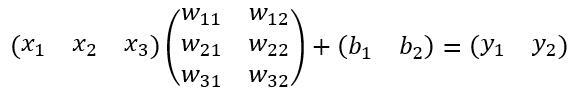
其中W和bias B都是预先训练好的，即大小是固定的，当然输入X和输出Y也就是固定大小。所以，这也就印证了之前Roi Pooling的必要性。到这里，我想其他内容已经很容易理解，不在赘述了。

5 Faster R-CNN训练

Faster R-CNN的训练，是在已经训练好的model（如VGG_CNN_M_1024，VGG，ZF）的基础上继续进行训练。实际中训练过程分为6个步骤：

在已经训练好的model上，训练RPN网络，对应stage1_rpn_train.pt
利用步骤1中训练好的RPN网络，收集proposals，对应rpn_test.pt
第一次训练Fast RCNN网络，对应stage1_fast_rcnn_train.pt
第二训练RPN网络，对应stage2_rpn_train.pt
再次利用步骤4中训练好的RPN网络，收集proposals，对应rpn_test.pt
第二次训练Fast RCNN网络，对应stage2_fast_rcnn_train.pt

可以看到训练过程类似于一种“迭代”的过程，不过只循环了2次。至于只循环了2次的原因是应为作者提到：”A similar alternating training can be run for more iterations, but we have observed negligible improvements”，即循环更多次没有提升了。接下来本章以上述6个步骤讲解训练过程。

下面是一张训练过程流程图，应该更加清晰。

&lt;img src=”https://pic1.zhimg.com/v2-ed3148b3b8bc3fbfc433c7af31fe67d5_b.jpg” data-size=”normal” class=”content_image”&gt;

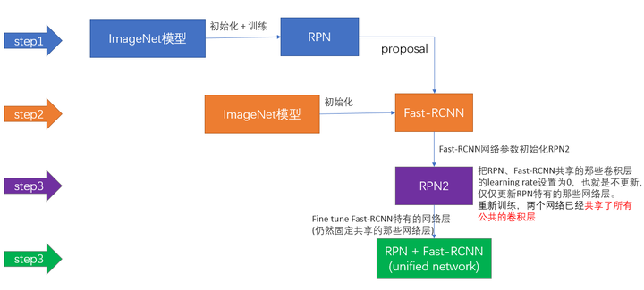图18 Faster RCNN训练步骤（引用自参考文章[1]）

5.1 训练RPN网络

在该步骤中，首先读取RBG提供的预训练好的model（本文使用VGG），开始迭代训练。来看看stage1_rpn_train.pt网络结构，如图19。

&lt;img src=”https://pic3.zhimg.com/v2-c39aef1d06e08e4e0cec96b10f50a779_b.jpg” data-size=”small” data-rawwidth=”1142″ data-rawheight=”899″ class=”origin_image zh-lightbox-thumb” width=”1142″ data-original=”https://pic3.zhimg.com/v2-c39aef1d06e08e4e0cec96b10f50a779_r.jpg”&gt;

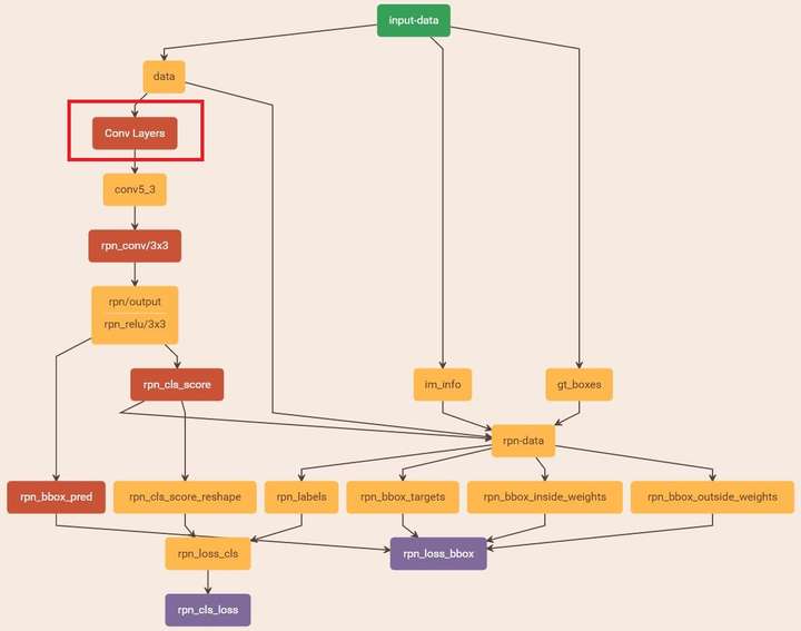图19 stage1_rpn_train.pt（考虑图片大小，Conv Layers中所有的层都画在一起了，如红圈所示，后续图都如此处理）

与检测网络类似的是，依然使用Conv Layers提取feature maps。整个网络使用的Loss如下：

&lt;img src=”https://pic3.zhimg.com/v2-1c964d29dadf51bfe82ec783344b899e_b.jpg” data-caption=”” data-size=”normal” data-rawwidth=”472″ data-rawheight=”175″ class=”origin_image zh-lightbox-thumb” width=”472″ data-original=”https://pic3.zhimg.com/v2-1c964d29dadf51bfe82ec783344b899e_r.jpg”&gt;

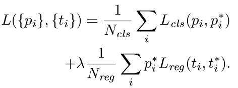
上述公式中，表示anchors index， $p_{i}$ 表示foreground softmax probability， $p_{i}^{*}$ 代表对应的GT predict概率（即当第i个anchor与GT间；反之时，认为是该anchor是background， $p_{i}^{*}=0$ ；至于那些的anchor则不参与训练）；代表predict bounding box， $t^{*}$ 代表对应foreground anchor对应的GT box。可以看到，整个Loss分为2部分：

cls loss，即rpn_cls_loss层计算的softmax loss，用于分类anchors为forground与background的网络训练
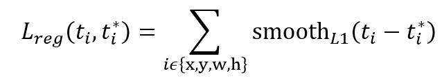
reg loss，即rpn_loss_bbox层计算的soomth L1 loss，用于bounding box regression网络训练。注意在该loss中乘了 $p_{i}^{*}$ ，相当于只关心foreground anchors的回归（其实在回归中也完全没必要去关心background）。

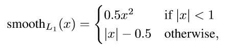
由于在实际过程中， $N_{cls}$ 和 $N_{reg}$ 差距过大，用参数λ平衡二者（如 $N_{cls}=256$ ， $N_{reg}=2400$ 时设置），使总的网络Loss计算过程中能够均匀考虑2种Loss。这里比较重要是 $L_{reg}$ 使用的soomth L1 loss，计算公式如下：

&lt;img src=”https://pic3.zhimg.com/v2-476fd71f83f92f9638d998c248bd9be2_b.jpg” data-caption=”” data-size=”normal” data-rawwidth=”638″ data-rawheight=”114″ class=”origin_image zh-lightbox-thumb” width=”638″ data-original=”https://pic3.zhimg.com/v2-476fd71f83f92f9638d998c248bd9be2_r.jpg”&gt;

&lt;img src=”https://pic3.zhimg.com/v2-0c13e37c2bb8e1a4f58361efb39a3795_b.jpg” data-caption=”” data-size=”normal” data-rawwidth=”462″ data-rawheight=”95″ class=”origin_image zh-lightbox-thumb” width=”462″ data-original=”https://pic3.zhimg.com/v2-0c13e37c2bb8e1a4f58361efb39a3795_r.jpg”&gt;

了解数学原理后，反过来看图18：

在RPN训练阶段，rpn-data（python AnchorTargetLayer）层会按照和test阶段Proposal层完全一样的方式生成Anchors用于训练
对于rpn_loss_cls，输入的rpn_cls_scors_reshape和rpn_labels分别对应与 $p^{*}$ ， $N_{cls}$ 参数隐含在与 $p^{*}$ 的caffe blob的大小中
对于rpn_loss_bbox，输入的rpn_bbox_pred和rpn_bbox_targets分别对应于 $t^{*}$ ，rpn_bbox_inside_weigths对应 $p^{*}$ ，rpn_bbox_outside_weigths未用到（从soomth_L1_Loss layer代码中可以看到），而 $N_{reg}$ 同样隐含在caffe blob大小中

这样，公式与代码就完全对应了。特别需要注意的是，在训练和检测阶段生成和存储anchors的顺序完全一样，这样训练结果才能被用于检测！

5.2 通过训练好的RPN网络收集proposals

在该步骤中，利用之前的RPN网络，获取proposal rois，同时获取foreground softmax probability，如图20，然后将获取的信息保存在python pickle文件中。该网络本质上和检测中的RPN网络一样，没有什么区别。

&lt;img src=”https://pic1.zhimg.com/v2-1ac5f8a2899ee413464ecf7866f8f840_b.jpg” data-size=”normal” data-rawwidth=”396″ data-rawheight=”726″ class=”content_image” width=”396″&gt;

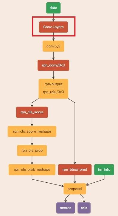图20 rpn_test.pt

5.3 训练Faster RCNN网络

读取之前保存的pickle文件，获取proposals与foreground probability。从data层输入网络。然后：

将提取的proposals作为rois传入网络，如图19蓝框
计算bbox_inside_weights+bbox_outside_weights，作用与RPN一样，传入soomth_L1_loss layer，如图20绿框

这样就可以训练最后的识别softmax与最终的bounding box regression了，如图21。

&lt;img src=”https://pic1.zhimg.com/v2-fbece817952865689187e68f0af86792_b.jpg” data-size=”small” data-rawwidth=”1248″ data-rawheight=”892″ class=”origin_image zh-lightbox-thumb” width=”1248″ data-original=”https://pic1.zhimg.com/v2-fbece817952865689187e68f0af86792_r.jpg”&gt;

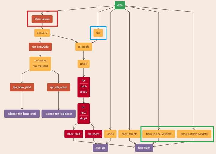图21 stage1_fast_rcnn_train.pt

之后的stage2训练都是大同小异，不再赘述了。Faster R-CNN还有一种end-to-end的训练方式，可以一次完成train，有兴趣请自己看作者GitHub吧。

参考文献：

- https://zhuanlan.zhihu.com/p/24916624
- Object Detection and Classification using R-CNNs

转载于:https://www.cnblogs.com/MY0213/p/9705669.html

发布者：全栈程序员-用户IM，转载请注明出处：https://javaforall.cn/101399.html原文链接：https://javaforall.cn

【正版授权，激活自己账号】： Jetbrains全家桶Ide使用，1年售后保障，每天仅需1毛

【官方授权正版激活】： 官方授权正版激活支持Jetbrains家族下所有IDE 使用个人JB账号...

1 Conv layers

2 Region Proposal Networks(RPN)

2.1 多通道图像卷积基础知识介绍

2.2 anchors

2.3 softmax判定foreground与background

2.4 bounding box regression原理

2.5 对proposals进行bounding box regression

2.6 Proposal Layer

3 RoI pooling

3.1 为何需要RoI Pooling

3.2 RoI Pooling原理

4 Classification

5 Faster R-CNN训练

5.1 训练RPN网络

5.2 通过训练好的RPN网络收集proposals

5.3 训练Faster RCNN网络

相关推荐

一个反射型XSS例子的解析

【主席树】bzoj3932 [CQOI2015]任务查询系统

java volatile关键字的作用_java volatile关键字作用及使用场景详解

linux .gz文件 解压缩命令的简单使用

ubuntu 更新源详细操作步骤「建议收藏」

爬虫之上传文件，request如何上传文件

发表回复

linux .gz文件解压缩命令的简单使用